
The sum of a normal and a truncated normal
(1) Background
Consider the sum of a normal \(Z_1 \sim N(\mu_1,\tau_1^2)\) and a truncated normal \(Z_2 \sim TN(\mu_2,\tau_2^2,a,b)\), denoted \(W=Z_1+Z_2\). How can this normal-truncated sum (NTS) be characterized? One approach for doing inference on \(W\) would be to simply sample from \(Z_1\) and \(Z_2\), which can be done with most statistical software. However, having an analytical or numerical method for calculating the density (PDF) and cumulative distribution (CDF) of \(W\) has several benefits over the sampling approach. This includes including vectorization, reproducibility across software programs, and faster compute times (especially for the tails of the distribution). This post will provide python code to calculate the PDF and CDF of an arbitrary NTS. The usefulness of this distribution will be highlighted in three instances: i) quality control, ii) two-stage hypothesis testing, and iii) data carving for selective inference.
This post will make extensive use of the theoretical results from Arnold et. al (1993) (hereafter Arnold) and Kim (2006) (hereafter Kim). Sections (2) and (3) are not original work, but instead show how to translate these research papers into usable code. In section (4) the two-stage hypothesis testing is an original contribution. Data carving is an established idea, but to my knowledge, no one has pointed out the relationship between data carving and the NTS distribution. In order to make this post more readable, the important classes are called in from a secondary file (e.g. NTS). One figure has made with R code. To replicate the entire pipeline, including figures, see here.
(2) Integrating a bivariate normal CDF
The CDF of a bivariate normal (BVN) will turn out to be necessary to calculate the CDF of an NTS. While there is no closed-form solution to the CDF of a BVN (unless the point of evaluation occurs at the origin), the integration problem can be quickly solved by numerical methods. Additionally, if the user is willing to accept a non-exact solution, there are approximation methods which yield an analytical solution that can be easily vectorized. This section will briefly review both approaches.
Following the notation of the literature, the orthant probability of a standard BVN[1], \(L(h,k,\rho)=P(X_1\geq h, X_2\geq k)\), is equivalent to solving the following integral introduced by Sheppard 130 years ago:
\[\begin{align} L(h,k,\rho) &= \frac{1}{2\pi\sqrt{1-\rho^2}} \int_h^\infty \int_k^\infty \exp \Bigg[ - \frac{x^2-2\rho x y + y^2}{2(1-\rho^2)} \Bigg] dx dy \\ &= \frac{1}{2\pi} \int_{\arccos(\rho)}^{\pi} \exp \Bigg[ - \frac{h^2+k^2-2hk\cos(\theta)}{2\sin^2(\theta)} \Bigg] d\theta \tag{1}\label{eq:sheppard} \end{align}\]Note that the orthant probability can easily be related to the CDF: \(F(h,k,\rho)=P(X_1\leq h, X_2\leq k) = L(h,k,\rho) + \Phi(h) + \Phi(k) - 1\). The CDF and PDF of a standard normal are denoted by \(\Phi(\cdot)\) and \(\phi(\cdot)\), respectively. What is interesting about \(\eqref{eq:sheppard}\) is that the problem of integrating out both \(X_1\) and \(X_2\) can been reduced to a single variable of integration.
In python, scipy.integrate.quad can be used to quickly solve \(\eqref{eq:sheppard}\). As will be shown, the method turns out to produce results identical to that of the scipy.stats.multivariate_normal.cdf function. Even though there is no closed-form solution, Cox 1991 showed that \(L(\cdot)\) could be approximated using a simple Taylor expansion.
Cox showed that this approximation method works well for reasonable ranges of \(\rho\) (absolute coefficient less than 90%). For users willing to trade off accuracy for speed, \(\eqref{eq:cox}\) allows for rapid vectorization cross different values of \(\rho\), \(h\), or \(k\). The code block below will use the BVN class to calculate the orthant probability and perform sampling.
# Modules needed for post
import numpy as np
import pandas as pd
from scipy.stats import norm
from statsmodels.stats.proportion import proportion_confint as propCI
from classes import BVN, NTS, two_stage, ols, dgp_yX, tnorm

mu = np.array([1,2])
sigma = np.array([0.5,2])
dist_BVN = BVN(mu,sigma,rho=0.4)
h, k = 2, 3
pval_scipy = dist_BVN.orthant(h, k, method='scipy')[0]
pval_sheppard = dist_BVN.orthant(h, k, method='sheppard')[0]
pval_cox = dist_BVN.orthant(h, k, method='cox')[0]
nsim = 1000000
pval_rvs = dist_BVN.rvs(nsim)
pval_rvs = pval_rvs[(pval_rvs[:,0]>h) & (pval_rvs[:,1]>k)].shape[0]/nsim
methods = ['scipy','sheppard','cox','rvs']
pvals = [pval_scipy, pval_sheppard, pval_cox, pval_rvs]
pd.DataFrame({'method':methods,'orthant':pvals})
| method | orthant | |
|---|---|---|
| 0 | scipy | 0.040615 |
| 1 | sheppard | 0.040615 |
| 2 | cox | 0.040670 |
| 3 | rvs | 0.040958 |
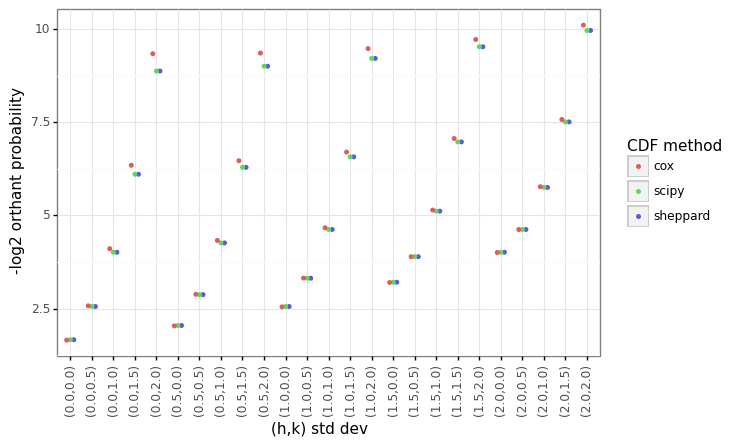
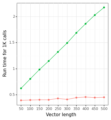
The output results show that using either the multivariate_normal (scipy) class or directly calling integration solvers (sheppard) produces identical results. Figure 1A below shows that the Cox-method is very close to the numerical solution, although there are no definitive error bounds (in Cox’s paper he found that the worst-case empirical error was around 10%). Although the figure is not shown, there is no improvement in the run time using the sheppard method over scipy’s built in MVN distribution for a single estimate, and scipy is faster over a matrix of values. There are substantial gains in the run time for vectorization across a matrix of \(h,k\) values using Cox’s methods (Figure 1B).
Figure 1: BVN comparison
| |
|
 |
 |
(3) Deriving the PDF and CDF
The first step to characterize the NTS distribution is to understand the distribution of a truncated bivariate normal distribution (TBVN).
\[\begin{align*} (X_1, X_2) &\sim \text{TBVN}(\theta, \Sigma, \rho, a, b) \\ E([X_1,X_2]) &= [\theta_1, \theta_2] \\ V([X_1,X_2]) &= \begin{pmatrix} \sigma_1^2 & \rho \sigma_1\sigma_2 \\ \rho \sigma_1\sigma_2 & \sigma_2^2 \end{pmatrix} \\ X_1 &\in \mathbb{R}, \hspace{3mm} X_2 \in [a,b] \end{align*}\]Notice that the TBVN takes the same formulation as a bivariate normal (a mean vector, a covariance matrix, and a correlation coefficient \(\rho\)) except that the random variable \(X_2\) term is bound between \(a\) and \(b\). Arnold showed that the marginal density of the non-truncated random variable \(X_1\) could be written as follows:
\[\begin{align} f_W(x) &= f_{X_1}(x) = \frac{\phi(m_1(x)) \Bigg[ \Phi\Big(\frac{\beta-\rho \cdot m_1(x)}{\sqrt{1-\rho^2}}\Big) - \Phi\Big(\frac{\alpha-\rho \cdot m_1(x)}{\sqrt{1-\rho^2}}\Big) \Bigg] }{\sigma_1\cdot Z} \tag{3}\label{eq:arnold} \\ m_1(x) &= (x - \theta_1)/\sigma_1 \\ \alpha &= \frac{a-\theta_2}{\sigma_2}, \hspace{3mm} \beta = \frac{b-\theta_2}{\sigma_2} \\ Z &= \Phi(\beta) - \Phi(\alpha) \end{align}\]Kim showed that an could be written as a TBVN by a simple change of variables:
\[\begin{align*} X_1 &= Z_1 + Z_2^u \\ X_2 &= Z_2^u, \hspace{3mm} X_2 \in [a,b] \\ Z_2^u &\sim N(\mu_2,\tau_2^2) \\ \theta &= [\mu_1 + \mu_2, \mu_2] \\ \Sigma &= \begin{pmatrix} \tau_1^2 + \tau_2^2 & \rho \sigma_1\sigma_2 \\ \rho \sigma_1\sigma_2 & \tau_2^2 \end{pmatrix} \\ \rho &= \sigma_2 / \sigma_1 = \tau_2/\sqrt{\tau_1^2 + \tau_2^2} \\ Z_1 + Z_2 &= W \sim NTS(\theta(\mu),\Sigma(\tau^2), a, b) \end{align*}\]Where \(Z^u_2\) is the non-truncated version of \(Z_2\). Clearly this specification of the TBVN is equivalent to the NTS and the marginal distribution of \(X_1\) is equivalent to the PDF of \(W\). Kim showed that the integral of \(\eqref{eq:arnold}\) was equivalent to solving the orthant probabilities of a standard BVN :
\[\begin{align} F_W &= F_{X_1}(x) = 1 - \frac{L(m_1(x),\alpha,\rho) - L(m_1(x),\beta,\rho)}{Z} \tag{4}\label{eq:kim} \end{align}\]Hence, the PDF for an can be solved analytically, and CDF can be solved using either numerical methods for the exact univariate integral in \(\eqref{eq:sheppard}\) or Cox’s approximation method in \(\eqref{eq:cox}\). The code for the NTS class has a pdf and cdf method needed to calculate \(\eqref{eq:arnold}\) and \(\eqref{eq:kim}\). The NTS class also provides a quantile function \(F^{-1}_W(p)=\sup_w F_W(w) \leq p\), although this function tends to be slow given it has to solve an optimization value for each queried percentage.
Next, let’s generate NTS data with the following parameters: \(\mu_1=1\), \(\tau_1=1\) (for \(Z_1\)), \(\mu_2=1\), \(\tau_2=2\), \(a=-1\), and \(b=4\) (for \(Z_2\)).
# Demonstrated with example
mu1, tau1 = 1, 1
mu2, tau2, a, b = 1, 2, -1, 4
mu, tau = np.array([mu1, mu2]), np.array([tau1,tau2])
dist_NTS = NTS(mu=mu,tau=tau, a=a, b=b)
n_iter = 100000
W_sim = dist_NTS.rvs(n=n_iter,seed=1)
mu_sim, mu_theory = W_sim.mean(),dist_NTS.mu_W
xx = np.linspace(-5*mu.sum(),5*mu.sum(),n_iter)
mu_quad = np.sum(xx*dist_NTS.pdf(xx)*(xx[1]-xx[0]))
methods = ['Empirical','Theory', 'Quadrature']
mus = [mu_sim, mu_theory, mu_quad]
# Compare
print(pd.DataFrame({'method':methods,'mu':mus}))
      method       mu
   Empirical  2.292354
      Theory  2.290375
  Quadrature  2.290375
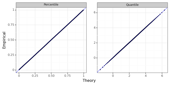
The output above compares the empirical mean of the simulated data with the sum of the two location parameters of \(Z_1\) and \(Z_2\), as well as what we would estimate using a quadrature procedure with equation \(\eqref{eq:arnold}\), as \(E(W)=\int w F_W(w) dw \approx \sum w F_W(w) dw\) for a small \(dw\). Next, we can compare the actual and theoretical percentiles and quantiles against the empirical ones seen from W_sim. As expected, they are visually indistinguishable from each other.[2]
Figure 2: NTS P-P & Q-Q plot
(4.A) Application: Quality control
In some manufacturing processes, one of the components may go through a quality control procedure that removes items above or below a certain threshold. For example, this question was posed in a 1964 issue of Technometrics:
An item which we make has, among others, two parts which are assembled additively with regard to length. The lengths of both parts are normally distributed but, before assembly, one of the parts is subjected to an inspection which removes all individuals below a specified length. As an example, suppose that X comes from a normal distribution with a mean 100 and a standard deviation of 6, and Y comes from a normal distribution with a mean of 50 and a standard deviation of 3, but with the restriction that Y > 44. How can I find the chance that X + Y is equal to or less than a given value?
Subsequent answers focused on value of \(P(X + Y < 138) \approx 0.03276\). We can confirm this by using the NTS class.
mu1, tau1 = 100, 6
mu2, tau2, a, b = 50, 3, 44, np.inf
mu, tau = np.array([mu1, mu2]), np.array([tau1,tau2])
dist_A = NTS(mu=mu,tau=tau, a=a, b=b)
print('P(X+Y<138)=%0.5f' % dist_A.cdf(138))
P(X+Y<138)=0.03276
(4.B) Two-stage testing
In a previous post I discussed a two-stage testing strategy designed to validate a machine learning regression model. The framework can be generalized as follows: 1) estimate an upper-bound on the mean of a Gaussian, 2) use this upper bound as the null hypothesis on a new sample of data.[3] This is useful in order to reject the null (in the second stage) to say the mean is at most some value. Several simplifying assumptions are made to make the analysis tractable: the data are IID and from the same normal distribution: \(S, T \overset{iid}{\sim} N(\delta,\sigma^2)\), and that \(n\) and \(m\) are large enough so that the difference between the normal and student-t distributions are sufficiently small. The statistical pipeline is as follows.
- Estimate the mean and variance on the first Gaussian sample
- Estimate the \(1-\gamma\) quantile of this distribution to set the null hypothesis
- Estimate mean and variance on second Gaussian sample
- Calculate a one-sided test statistic
When the null is true, then the estimate of the upper bound is too low because \(\delta\) is larger than what we estimate (\(\hat{\delta}_0\)). Concomitantly, the null being false implies that we have successfully bounded the actual mean. If \(\gamma >0.5\), then \(E(s)<0\) because \(\hat{\delta}_0\) will tend to be above the true average of \(\delta\). The statistical information provided by this procedure is two-fold. First, \(\delta_0\) has the property that it will be larger than the true mean \((1-\gamma)\)% of the time.[4] Second, when the null is false (i.e. the bound holds) we will be able to compute the power in advance. Now, where does the NTS fit into this? In order to bound the type-I error rate to \(\alpha\), we need to know the distribution of \(s\) when the null is true: \(\delta > \hat{\delta}_0\):
\[\begin{align*} \hat{s} &= \frac{\hat{\delta}_T - \delta}{\hat{\sigma}_m} - \frac{\hat{\delta}_0 - \delta}{\hat{\sigma}_m} \hspace{2mm} \Big| \hspace{2mm} \hat{\delta}_0 > \delta \\ &= N(0,1) - \frac{\hat{\delta}_S-\delta + \hat{\sigma}_n\cdot\Phi^{-1}_{1-\gamma}}{\hat{\sigma}_m} \hspace{2mm} \Big| \hspace{2mm} \hat{\delta}_S + \hat{\sigma}_n\cdot\Phi^{-1}_{1-\gamma} - \delta > 0 \\ &= N(0,1) + TN\big( - \sqrt{m/n} \cdot \Phi^{-1}_{1-\gamma}, m/n, 0, \infty \big) \end{align*}\]Hence the critical value \(t_\alpha = F^{-1}_W(\alpha)\) can be found by inverting \(\eqref{eq:kim}\) (i.e. the quantile function) with the following parameters from our original notation:
\[\begin{align*} \mu &= \big[ 0, - \sqrt{m/n} \cdot \Phi^{-1}_{1-\gamma}\big] \\ \tau^2 &= \big[1, m/n \big] \\ \hat{s} | H_0 &\sim NTS(\theta(\mu), \Sigma(\tau^2), 0, \infty ) \\ \hat{s} | H_A &\sim NTS(\theta(\mu), \Sigma(\tau^2), -\infty, 0 ) \end{align*}\]Notice that the distribution of the NTS test statistic only depends on \(m\), \(n\), and \(\gamma\) as the test statistic \(s\) is a pivot over all possible values of \(\delta\) or \(\sigma\) (which are nuisance parameters). This means that the researcher can calculate the critical value \(t_\alpha\) as well as estimate the power \(1-\beta = P(\hat s < t_{\alpha})\) in advance of the data. To the extent that there are degrees of freedom in selecting \(m\), \(n\), and \(\gamma\), several trade-offs occur.
- Smaller values of \(\gamma\) (keeping \(m\) and \(n\) fixed) increase power but lower statistical information with a higher average upper bound
- Higher values of \(n\) (keeping \(m\) and \(\gamma\) fixed) reduce power but increase statistical information with a lower average upper bound
- Higher values of \(m\) (keeping \(n\) and \(\gamma\) fixed) increase statistical power
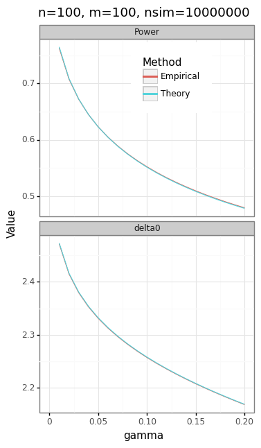
If \(m+n=k\) is fixed, then a trade-off can be made between the size of the upper bound from the first stage, and the power in the second stage. The simulations below check that the \(\hat{s}\) is characterized by an distribution, and examine how the power and statistical information of the test varies for the following parameters: \(\delta=2\), \(\sigma^2=4\), \(n+m=200\), \(\gamma=0.01\), and \(\alpha=0.05\).
delta, sigma2 = 2, 4
n, m = 100, 100
gamma, alpha = 0.01, 0.05
nsim = 10000000
p_seq = np.round(np.arange(0.01,1,0.01),2)
two_stage(n=n, m=m, gamma=gamma, alpha=alpha, pool=True).power

# --- (A) CALCULATE N=M=100 PP-QQ PLOT --- #
dist_2s = two_stage(n=n, m=m, gamma=gamma, alpha=alpha, pool=True)
df_2s = dist_2s.rvs(nsim=nsim, delta=delta, sigma2=sigma2)
df_2s = df_2s.assign(Null=lambda x: x.d0hat < delta)
df_2s = df_2s.assign(reject=lambda x: x.shat < dist_2s.t_alpha)

qq_emp = df_2s.groupby('Null').apply(lambda x: pd.DataFrame({'pp':p_seq,'qq':np.quantile(x.shat,p_seq)}))
qq_emp = qq_emp.reset_index().drop(columns='level_1')
qq_theory_H0 = dist_2s.H0.ppf(p_seq)
qq_theory_HA = dist_2s.HA.ppf(p_seq)
tmp1 = pd.DataFrame({'pp':p_seq,'theory':qq_theory_H0,'Null':True})
tmp2 = pd.DataFrame({'pp':p_seq,'theory':qq_theory_HA,'Null':False})
qq_pp = qq_emp.merge(pd.concat([tmp1, tmp2]))
qq_pp = qq_pp.melt(['pp','Null'],['qq','theory'],'tt')

# --- (B) POWER AS GAMMA VARIES --- #
gamma_seq = np.round(np.arange(0.01,0.21,0.01),2)
power_theory = np.array([two_stage(n=n, m=m, gamma=g, alpha=alpha, pool=False).power for g in gamma_seq])
ub_theory = delta + np.sqrt(sigma2/n)*t(df=n-1).ppf(1-gamma_seq)
power_emp, ub_emp = np.zeros(power_theory.shape), np.zeros(ub_theory.shape)
for i, g in enumerate(gamma_seq):
    tmp_dist = two_stage(n=n, m=m, gamma=g, alpha=alpha, pool=False)
    tmp_sim = tmp_dist.rvs(nsim=nsim, delta=delta, sigma2=sigma2)
    tmp_sim = tmp_sim.assign(Null=lambda x: x.d0hat < delta,
                reject=lambda x: x.shat < tmp_dist.t_alpha)
    power_emp[i] = tmp_sim.query('Null==False').reject.mean()
    ub_emp[i] = tmp_sim.d0hat.mean()

tmp1 = pd.DataFrame({'tt':'theory','gamma':gamma_seq,'power':power_theory,'ub':ub_theory})
tmp2 = pd.DataFrame({'tt':'emp','gamma':gamma_seq,'power':power_emp,'ub':ub_emp})
dat_gamma = pd.concat([tmp1, tmp2]).melt(['tt','gamma'],None,'msr')

# --- (C) POWER AS N = K - M VARIES --- #

k = n + m
n_seq = np.arange(5,k,5)
dat_nm = pd.concat([pd.DataFrame({'n':nn,'m':k-nn,
    'power':two_stage(n=nn, m=k-nn, gamma=gamma, alpha=alpha, pool=True).power},index=[nn]) for nn in n_seq])
dat_nm = dat_nm.reset_index(None,True).assign(ub=delta + np.sqrt(sigma2/n_seq)*t(df=n_seq-1).ppf(1-gamma))
dat_nm = dat_nm.melt(['n','m'],None,'msr')
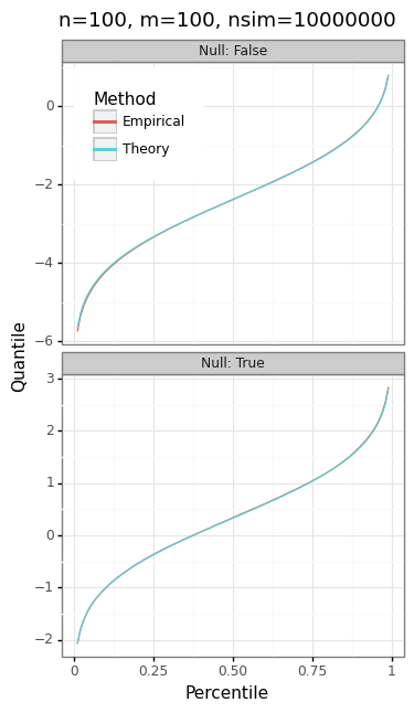
Figure 3: Two-stage test statistic
| |
|
|
 |
 |
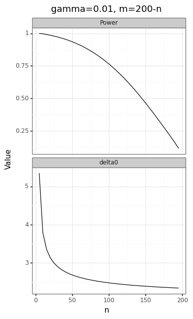 |
The panel of plots in Figure 3 shows the trade-offs inherent in the choice of \(m\), \(n\), and \(\gamma\). Because the actual and expected quantiles line up perfectly (Figure 3A), we can be confident that the NTS distribution correctly describes the two-stage test statistic.
(4.C) Application: Data carving
The classical instruments of statistical inference like p-values and confidence internals have probabilistic properties whose validity relies on an a priori specification of the model and null hypotheses. Which variables will be tested, and through which model, must be determined independent of any data. In the age of exploratory statistics and large datasets these assumptions are increasingly at odds with empirical practice. For example, researchers who use a lasso model to find a sparse set of coefficients will often “investigate” the importance of the features by examining the frequency of which variables get selected through bootstrapping or cross-validation.[5] Unfortunately, the traditional methods of doing inference on the coefficients of a regression model do not work for the lasso because which coefficients get selected is a function of the data. In other words, both the model and the null hypothesis is determined ex post rather than a priori.
In the framework of Fithian, Sun, and Taylor (see Optimal Inference After Model Selection), obtaining valid inference in the adaptive selection paradigm requires a two-stage process: “1) the selection stage determines what questions to ask, and 2) the inference stage answers those questions.” Specifically, we are interested in “selective validity,” that is obtaining the right level of a test conditional on selection process.
For multiple regression or multiple comparison tests, selection usually amounts to restricting hypothesis testing to parameters that exceed some value. For example, in genetics, we may only want to examine genes whose association with a phenotype has a z-score (in absolute value) greater than 2. In the case of the lasso, we want to obtain confidence intervals for the features with non-zero coefficients in the model. When the distribution of these test statistics is Gaussian, then conditioning on the selection event usually leads to a truncated Gaussian distribution.
Three statistical approaches that yield selective validity include:
- Data splitting
- Selective inference
- Data carving
The idea of using a portion of the data to come up with hypotheses, and then another portion to carry out inference, has been an accepted practice amongst statisticians for decades (see Cox (1975)). If data splitting is done properly, then its inferences must be valid in the classical sense because the unused portion of the data is truly independent. The downside of data splitting is twofold. First, it suffers from a “p-value lottery”, so that the results will vary depending on which random seed is used. Second, the portion of the data that is used for selection will contain unused statistical information that needs to be discarded. For example, suppose the selection procedure only selects parameters that have a z-score greater than 0.01 for second-stage inference. Under the null of no effect, this will discard less than 1% of hypotheses, which means that the selection procedure is effectively toothless. But for the inference in stage two to be valid, this portion of the dataset needs to be discarded regardless. The amount of residual statistical information leftover from the selection stage will be inversely proportional to the stringency of the selection procedure.
The selective inference approach conditions on the selection event and then does inference on the “remaining” portion of the statistical information. Nevertheless, there is an inherent selection-inference trade-off between data splitting and selective inference, with the latter finding more interesting models/hypotheses but at the expense of lower power.
A middle-ground between data splitting and selective inference is data carving, which carries out inference with a combination of an unused portion of the data as well as the remaining information from the data that was already used for selective inference.
Data carving will necessarily have a higher power than selective inference because the unused portion of the data does not need to be conditioned on. However, selective inference is more likely to find interesting hypotheses because the entire dataset is used during the selection stage. When deciding how much data to set aside to inference, the researcher must balance the need for power versus selection. Selective inference is the case of data carving when the fraction of unused data approaches zero. However, data carving always dominates data splitting for the same fraction of data used for the inference stage because data carving throws away only the statistical information implied by the selection procedure on the selection stage, whereas data splitting completely discards the information.
The classical linear model is has a Gaussian likelihood when it is unconditioned, and a truncated Gaussian when the coefficients have some conditioning event. The combination of these two estimators (data carving) therefore amounts to an.
Suppose we have \(n\) paired observations of an outcome and a feature set: \((\by,\bX)=((y_1,\bx_1),\dots,(y_n,\bx_n))\). Assume that \(y_i \sim N(\mu_i, \sigma^2)\), where \(\mu_i = \bx_i^T\bbeta\), with a known variance \(\sigma^2\).[6] We are only interesting in carrying out inference on the coefficients whose absolute magnitude is at least 0.1. In the data splitting case we use the first \(m<n\) samples of the data to obtain the least squares estimate and then do inference on the features with a sufficiently large (absolute) coefficient on the remaining \(k=n-m\) samples:
\[\begin{align*} &\text{Data splitting inference} \\ \bhat^m &= (\bX_m^T\bX_m)^{-1}\bX_m^T\by_m \\ S_m &= \{| \bhat_{j,S_m} | \geq 0.1 \} \\ \bhato &= (\bX_{k,S_m}^T\bX_{k,S_m})^{-1}\bX_{k,S_m}^T\by \sim \text{MVN}(\beta_{S_m}, V_{k,S_m}) \\ V_{k,S_m} &= \sigma^2 (\bX_{k,S_m}^T\bX_{k,S_m})^{-1} \\ \bhato_j &\sim \begin{cases} N(\beta_j, [V_{k,S_m}]_{jj} ) & \text{ if } j\in S_m \\ \text{undefined} & \text{ if } j \not\in S_m \end{cases} \end{align*}\]In selective inference we do inference on the unused statistical information of the selection event, which amounts to a truncated Gaussian.
\[\begin{align*} &\text{Selective inference}\\ \bhat &= (\bX^T\bX)^{-1}\bX^T\by \\ S &= \{| \bhat_j | \geq 0.1 \} \\ \bhats_j &= \bhat_j | |\bhat_j| > 0.1 \hspace{3mm} \text{ if } j \in S \\ &\sim \begin{cases} TN(\beta_j,V_{jj},0.1,\infty) & \text{ if } \bhat_j\geq 0 \\ TN(\beta_j,V_{jj},-\infty,-0.1) & \text{ if } \bhat_j<0 \end{cases} \end{align*}\]The data carving estimator is a sum of these estimators indexed by the number of samples used for both:
\[\begin{align*} &\text{Data carving} \\ \bhatc_j &= \big( \bhat_j^m||\bhat_j^m|>0.1 \big) + \bhat_j^k \hspace{3mm} \text{ if } j \in S_m \\ &\sim \begin{cases} TN(\beta_j, [V_m]_{jj},0.1,\infty) + N(\beta_j, [V_{k,S_m}]_{jj}) & \text{ if } \bhat_j^m \geq 0 \\ TN(\beta_j, [V_m]_{jj},-\infty,-0.1) + N(\beta_j, [V_{k,S_m}]_{jj}) & \text{ if } \bhat_j^m < 0 \end{cases} \end{align*}\]For any null hypothesis \(\beta_j^0\), we can calculate the p-values and confidence intervals of \(\bhat_j\) for either approach at the \(1-\alpha\) level:
\[\begin{align*} \text{P-value}(\bhat_j) &= \begin{cases} 2\cdot \min\big\{ F_{\beta_j^0,V_{jj}^{1/2}}(|\bhat_j|), 1-F_{\beta_j^0,V_{jj}^{1/2}}(|\bhat_j|) \big\} & \text{ for data splitting} \\ 2\cdot \min\big\{ F_{\beta_j^0,V_{jj}^{1/2}}^{1,\infty}(|\bhat_j|), 1-F_{\beta_j^0,V_{jj}^{1/2}}^{1,\infty}(|\bhat_j|) \big\} & \text{ for selective inference and data carving} \\ \end{cases} \\ \text{CI lower bound}(\bhat_j) &= \begin{cases} \sup_\theta \{\theta: F_{\theta,V_{jj}^{1/2}}(\bhat_j) \geq 1-\alpha/2 \} & \text{ for data splitting} \\ \sup_\theta \{\theta: F_{\theta,V_{jj}^{1/2}}^{1,\infty}(\bhat_j) \geq 1-\alpha/2 \} & \text{ for selective inference data carving} \\ \end{cases} \\ \text{CI upper bound}(\bhat_j) &= \begin{cases} \inf_\theta \{\theta: F_{\theta,V_{jj}^{1/2}}(\bhat_j) \leq \alpha/2 \} & \text{ for data splitting data carving} \\ \inf_\theta \{\theta: F_{\theta,V_{jj}^{1/2}}^{1,\infty}(\bhat_j) \leq \alpha/2 \} & \text{ for selective inference data carving} \\ \end{cases} \end{align*}\]Where \(F_{a,b}^{c,d}\) denotes the CDF of a truncated normal or NTS with a mean and variance of \(a\) and \(b\), over a support of \([c,b]\) (I’m reusing the notation, as both distributions are indexed by four parameters). \(F_{a,b}\) is the CDF of a normal. In order for there to be identifiability in the case of an NTS, it will be assumed that \(\theta_1 = \theta_2\), since there are two means that go into the NTS. To make sure that the CI attributes work for the tnorm and NTS distribution, we should expect the intervals to exactly cover a mean parameter of zero at the 95% level when we observe the 2.5% and 97.5% quantile.
dist_TN = tnorm(mu=0, sig2=0.01, a=0.1, b=np.inf)
dist_NTS = NTS(mu=[0,0],tau=[0.1,0.1],a=0.1,b=np.inf)
p_sig = np.array([alpha/2, 1-alpha/2])
q_sig_TN = dist_TN.ppf(p_sig)
q_sig_NTS = dist_NTS.ppf(p_sig)
lb_TN = dist_TN.CI(q_sig_TN,gamma=1-alpha/2)
ub_TN = dist_TN.CI(q_sig_TN,gamma=alpha/2)
lb_NTS = np.array([dist_NTS.CI(q,gamma=1-alpha/2)[0] for q in q_sig_NTS])
ub_NTS = np.array([dist_NTS.CI(q,gamma=alpha/2)[0] for q in q_sig_NTS])
res1 = pd.DataFrame({'dist':'TN','lb':lb_TN,'ub':ub_TN})
res2 = pd.DataFrame({'dist':'NTS','lb':lb_NTS,'ub':ub_NTS})
res_CI = pd.concat([res1,res2]).reset_index(None,True)
res_CI.round(3)
| dist | lb | ub | |
|---|---|---|---|
| 0 | TN | -22.062 | -0.001 |
| 1 | TN | 0.000 | 0.461 |
| 2 | NTS | -0.377 | 0.000 |
| 3 | NTS | 0.000 | 0.318 |
One useful feature of both a truncated normal and an NTS is that the positive portion of the truncated distribution can be used for inference calculations as long as the truncation points are symmetric. This allows for an easier way to calculate CIs, keeping in mind that the lower and upper bounds will need to be swapped and multiplied by -1 after they are generated for negative coefficients.
dist_TN = tnorm(mu=0, sig2=0.01, a=-np.inf, b=-0.1)
dist_NTS = NTS(mu=[0,0],tau=[0.1,0.1], a=-np.inf, b=-0.1)
p_sig = np.array([alpha/2, 1-alpha/2])
q_sig_TN_neg = dist_TN.ppf(p_sig)
q_sig_NTS_neg = dist_NTS.ppf(p_sig)
sign1 = pd.DataFrame({'dist':'TN','q_pos':q_sig_TN,'q_neg':q_sig_TN_neg})
sign2 = pd.DataFrame({'dist':'NTS','q_pos':q_sig_NTS,'q_neg':q_sig_NTS_neg})
pd.concat([sign1,sign2]).reset_index(None,True).round(3)
| dist | q_pos | q_neg | |
|---|---|---|---|
| 0 | TN | 0.102 | -0.265 |
| 1 | TN | 0.265 | -0.102 |
| 2 | NTS | -0.058 | -0.372 |
| 3 | NTS | 0.372 | 0.058 |
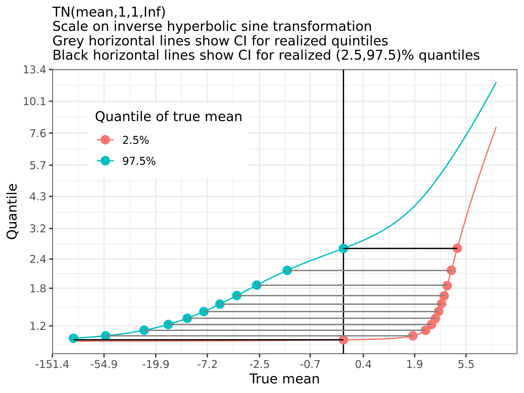
Unlike the truncated normal, the NTS intervals are roughly symmetric. Figure 4 shows what happens to the CIs for a truncated Gaussian as the observed point approaches the lower bound limit. Even though the CIs are valid and exact in that they provide the right nominal coverage \(P([L,U]\in \mu) = 1-\alpha)\), the amount of statistical information provided by these intervals becomes increasingly useless as the observed point reaches the truncation limit (and the remaining statistical information approaches zero).
Figure 4: Truncated normal confidence intervals
Now that we’ve shown that the CIs should contain the true mean parameter (or sum of equal means in the case of NTS), we can run the simulations on the OLS estimator for the different approaches. In each simulation the true coefficients will be zero, so that we can see the distribution of the estimator under a null hypothesis of no effect. Also, the variance of the response \(\sigma^2\) will assumed to be known. We should expect that CIs will cover the true mean (zero) 95% of the time, and the p-values will be less than 0.05, 5% of the time. Because only 1000 simulations are run, there will still be some variation in the coverage/rejection probabilities, but these will be shown to be within the normal range of measurement error.
cutoff = 0.1
n, p, sig2 = 100, 20, 1
m = int(n/2)

beta_null = np.repeat(0, p)
nsim = 1000
holder_SI, holder_ols, holder_carv = [], [], []
np.random.seed(nsim)
for i in range(nsim):
    if (i+1) % 100 == 0:
        print(i+1)
    resp, xx = dgp_yX(n=n, p=p, snr=1, b0=0, seed=i)
    # (i) Data splitting
    mdl1 = ols(y=resp[:m], X=xx[:m], has_int=False, sig2=sig2)
    abhat1 = np.abs(mdl1.bhat)
    M1 = abhat1 > cutoff
    if M1.sum() > 0:
        mdl2 = ols(y=resp[m:], X=xx[m:,M1], has_int=False, sig2=sig2)
        tmp_ols = pd.DataFrame({'sim':i,'bhat':mdl2.bhat,'Vjj':np.diagonal(mdl2.covar)})
        holder_ols.append(tmp_ols)
    # (iii) Data carving
    if M1.sum() > 0:
        tmp_carv = pd.DataFrame({'sim':i,'bhat1':mdl1.bhat[M1],'bhat2':mdl2.bhat,
                      'Vm':np.diagonal(mdl1.covar)[M1],'Vk':np.diagonal(mdl2.covar)})
        holder_carv.append(tmp_carv)
    # (ii) Selective inference
    mdl = ols(y=resp, X=xx, has_int=False, sig2=sig2)
    M = np.abs(mdl.bhat)>cutoff
    if M.sum() > 0:
        tmp_M = pd.DataFrame({'sim':i,'bhat':mdl.bhat[M],'Vjj':np.diagonal(mdl.covar)[M]})
    holder_SI.append(tmp_M)
# In NTS?
dat_NTS = pd.concat(holder_carv).reset_index(None,True).assign(tt='NTS')
# dat_NTS = dat_NTS.assign(pval=np.NaN,lb=np.NaN,ub=np.NaN)
# Assume we're in positive region, and then swap for negative signs
a_seq = np.repeat(cutoff, len(dat_NTS))
b_seq = np.repeat(np.inf, len(dat_NTS))
tau_seq = np.sqrt(np.c_[dat_NTS.Vk, dat_NTS.Vm])
mu_seq = np.zeros(tau_seq.shape)
dist_H0_NTS = NTS(mu_seq, tau_seq, a_seq, b_seq)
bhat12 = (dat_NTS.bhat1.abs() + dat_NTS.bhat2).values
pval_NTS = dist_H0_NTS.cdf(bhat12)
pval_NTS = 2*np.minimum(pval_NTS,1-pval_NTS)
assert np.abs(alpha - np.mean(pval_NTS < alpha)) < 2*np.sqrt(alpha*(1-alpha) / len(dat_NTS))
ub_NTS = dist_H0_NTS.CI(bhat12,gamma=alpha/2,nline=10,verbose=True)
lb_NTS = dist_H0_NTS.CI(bhat12,gamma=1-alpha/2,nline=10,verbose=True)
tmp_plu = pd.DataFrame(np.c_[np.sign(dat_NTS.bhat1),pval_NTS, lb_NTS, ub_NTS],columns=['sbhat','pval','lb','ub'])
tmp_plu.loc[tmp_plu.sbhat==-1,['lb','ub']] = (-1*tmp_plu.loc[tmp_plu.sbhat==-1,['lb','ub']]).iloc[:,[1,0]].values
tmp_plu = tmp_plu.assign(reject=lambda x: x.pval<alpha, cover=lambda x: np.sign(x.lb)!=np.sign(x.ub))
dat_NTS_inf = pd.concat([dat_NTS,tmp_plu[['lb','ub','reject','cover']]],1)

# Coverage for OLS
dat_ols = pd.concat(holder_ols).reset_index(None,True).assign(tt='OLS')
pval_ols = norm(loc=0,scale=np.sqrt(dat_ols.Vjj)).cdf(dat_ols.bhat)
pval_ols = 2*np.minimum(pval_ols,1-pval_ols)
CI_ols = cvec(dat_ols.bhat) + np.array([-1,1])*cvec(norm.ppf(1-alpha/2)*np.sqrt(dat_ols.Vjj))
dat_ols = dat_ols.assign(reject=pval_ols<alpha,cover=np.sign(CI_ols).sum(1)==0)

# Is truncated Gaussian?
dat_TN = pd.concat(holder_SI).assign(tt='TN')
dat_TN = dat_TN.assign(abhat=lambda x: x.bhat.abs(),
                       sbhat=lambda x: np.sign(x.bhat).astype(int))
dat_TN = dat_TN.sort_values('abhat',ascending=False).reset_index(None,True)
dist_TN_ols = tnorm(mu=0,sig2=dat_TN.Vjj.values,a=cutoff,b=np.inf)
pval_TN = dist_TN_ols.cdf(dat_TN.abhat)
pval_TN = 2*np.minimum(pval_TN,1-pval_TN)
dat_TN['pval'] = pval_TN
lb_TN = dist_TN_ols.CI(x=dat_TN.abhat.values,gamma=1-alpha/2,verbose=True,tol=1e-2)
ub_TN = dist_TN_ols.CI(x=dat_TN.abhat.values,gamma=alpha/2,verbose=True,tol=1e-2)
CI_TN = np.c_[lb_TN, ub_TN]
dat_TN = dat_TN.assign(reject=pval_TN<0.05, cover=np.sign(CI_TN).sum(1)==0)

cn_sub = ['sim','tt','reject','cover']
# Save data for later
dat_bhat = pd.concat([dat_TN[cn_sub], dat_ols[cn_sub],dat_NTS_inf[cn_sub]],0).reset_index(None,True)
res_NTS = dat_bhat.melt('tt',['reject','cover'],'msr').groupby(['tt','msr'])
res_NTS = res_NTS.value.apply(lambda x: pd.DataFrame({'p':x.mean(),'s':x.sum(),'n':len(x)},index=[0])).reset_index()
res_NTS = pd.concat([res_NTS,pd.concat(propCI(res_NTS.s,res_NTS.n,alpha,'beta'),1)],1)
res_NTS = res_NTS.rename(columns={0:'lb',1:'ub'}).drop(columns='level_2')
Figure 5: Coverage properties for three approaches
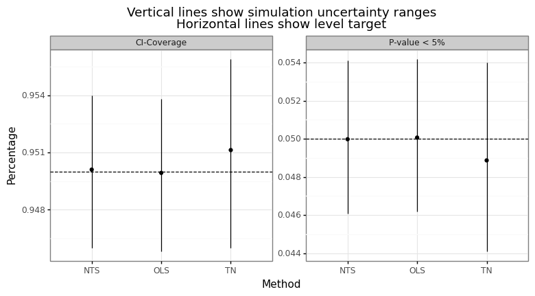
As expected, the p-values and CIs have the right nominal coverage. This gives us confidence that the NTS class can be used for more general data carving applications when the portion of the data that is used for inference is Gaussian, whilst the portion of the data that is used for selection yields a truncated Gaussian.
Footnotes
-
A standard BVN means that the means are zero, and the covariance matrix has a value of one on the diagonals and \(\rho\) on the off-diagonals. ↩
-
In reality, there are slight differences, they just cannot be seen on the figure. ↩
-
A lower bound can be studied just as easily as an upper bound. ↩
-
This is only true in the frequentist sense. We can say nothing about any one realization of \(\hat{\delta}_0\) itself, only about the random variable \(\delta_0\) in general. ↩
-
Here are just three examples of papers that use this frequency property found from the first page of a google search: here, here, and here. ↩
-
In practice \(\sigma^2\) needs to be estimated, which will make the classical distribution a student’s-t distribution rather than a normal, but this issue is ignored for convenience. ↩