
Confidence interval approximations for the AUROC
The area under the receiver operating characteristic curve (AUROC) is one of the most commonly used performance metrics for binary classification. Visually, the AUROC is the integral between the sensitivity and false positive rate curves across all thresholds for a binary classifier. The AUROC can also be shown to be equivalent to an instance of the Mann-Whitney-U test (MNU), a non-parametric rank-based statistic. This post addresses two challenges when doing statistical testing for the AUROC: i) how to speed up the calculation of the statistic, and ii) which inference procedure to use to obtain the best possible coverage. The AUROC’s relationship to the MNU will be shown to be important for both speed ups in calculation and resampling approaches for the bootstrap.
(1) Methods for calculating the AUROC
In the binary classification paradigm, a model produces a score associated with the probability that an observation belongs to class 1 (as opposed to class 0). The AUROC of any model is a probabilistic term: \(P(s^1 > s^0)\), where \(s^k\) is the distribution of scores from the model for class \(k\). In practice the AUROC is never known because the distribution of data is unknown! However, an unbiased estimate of the AUROC (a.k.a the empirical AUROC) can be calculated through one of several approaches.
The first method is to plot the ROC curve by measuring the sensitivity/specificity across all thresholds, and then use the trapezoidal rule for calculating the integral. This approach is computationally inefficient and should only be done for visualization purposes. A second method to obtain the empirical AUROC is to simply calculate the percentage of times the positive class score exceeds the negative class score:
\[\begin{align} AUC &= \frac{1}{n_1n_0} \sum_{i: y_i=1} \sum_{j: y_j=0} I(s_i > s_j) + 0.5\cdot I(s_i = s_j) \tag{1}\label{eq:auc_pair} \end{align}\]Where \(y_i\) is the binary label for the \(i^{th}\) observation and \(n_k\) is the number of instances for class \(k\). If we assume that the positive class is some fraction of the observation in the population: \(P(y=1) = \pi\), then on average, calculating the AUROC via \eqref{eq:auc_pair} requires \(\pi(1-\pi)n^2\) operations which means \(O(AUC)=n^2\). For larger sample sizes this quadratic complexity will lead to long run times. One method to bound the computational complexity of \eqref{eq:auc_pair} is to randomly sample, with replacement, \(m\) samples from each class of the data to get a stochastic approximation of the AUC.
\[\begin{align} sAUC &= \frac{1}{m} \sum_{i} P(\tilde{s_i}^1 > \tilde{s_i}^0) \tag{2}\label{eq:auc_rand} \end{align}\]Where \(\tilde{s_i}^k\) is a random instance from the scores of class \(k\). The stochastic AUROC approach has the nice computational advantage that it is \(O(m)\). As with other stochastic methods, \eqref{eq:auc_rand} requires knowledge of the sampling variation of the statistic, as well as seeding, which tends to discourage its use in practice. The third approach is to use the rank order of the data to calculate the empirical AUROC.
\[\begin{align} rAUC &= \frac{1}{n_1n_0} \sum_{i: y_i=1} r_i - \frac{n_1(n_1 +1)}{2} \tag{3}\label{eq:auc_rank} \end{align}\]Where \(r_i\) is the sample rank of the data. Since ranking a vector is \(O(n\log n)\), the computational complexity of \eqref{eq:auc_rank} is linearithmic, which will mean significant speed ups over \eqref{eq:auc_pair}.
(2) Run-time comparisons
The code block below shows the run-times for the different approaches to calculate the AUROC from section (1) across different sample sizes (\(n\)) with different positive class proportions (\(n_1/n\)). The stochastic approach uses \(m = 5 n\). It is easy to generate data from two distributions so that the population AUROC can be known in advance. For example, if \(s^1\) and \(s^0\) come from the normal distribution:
\[\begin{align*} s_i^0 \sim N(0,1)&, \hspace{2mm} s_i^1 \sim N(\mu,1), \hspace{2mm} \mu \geq 0, \\ P(s_i^1 > s_i^0) &= \Phi\big(\mu / \sqrt{2}\big). \end{align*}\]Alternatively one could use two exponential distributions:
\[\begin{align*} s_i^0 \sim Exp(1)&, \hspace{2mm} s_i^1 \sim Exp(\lambda^{-1}), \hspace{2mm} \lambda \geq 1, \\ P(s_i^1 > s_i^0) &= \frac{\lambda}{1+\lambda}. \end{align*}\]It is easy to see that scale parameter of the normal or exponential distribution can determined a priori to match some pre-specific AUROC target.
\[\begin{align*} \mu^* &= \sqrt{2} \cdot \Phi^{-1}(AUC) \\ \lambda^* &= \frac{AUC}{1-AUC} \end{align*}\]The simulations in this post will use the normal distribution for simplicity, although using the exponential distribution will not change the results of the analysis. The reason is that the variance of the AUROC will be identical regardless of the distribution that generated it, as long as those two distributions have the same AUROC.
"""
DEFINE HELPER FUNCTIONS NEEDED THROUGHOUT POST
"""

import os
import numpy as np
import pandas as pd
import plotnine
from plotnine import *
from scipy import stats
from scipy.interpolate import UnivariateSpline
from timeit import timeit
from sklearn.metrics import roc_curve, auc

def rvec(x):
    return np.atleast_2d(x)

def cvec(x):
    return rvec(x).T

def auc_pair(y, s):
    s1, s0 = s[y == 1], s[y == 0]
    n1, n0 = len(s1), len(s0)
    count = 0
    for i in range(n1):
        count += np.sum(s1[i] > s0)
        count += 0.5*np.sum(s1[i] == s0)
    return count/(n1*n0)

def auc_rand(y, s, m):
    s1 = np.random.choice(s[y == 1], m, replace=True)
    s0 = np.random.choice(s[y == 0], m, replace=True)
    return np.mean(s1 > s0)

def auc_rank(y, s):
    n1 = sum(y)
    n0 = len(y) - n1
    den = n0 * n1
    num = sum(stats.rankdata(s)[y == 1]) - n1*(n1+1)/2
    return num / den

def dgp_auc(n, p, param, dist='normal'):
    n1 = np.random.binomial(n,p)
    n0 = n - n1
    if dist == 'normal':
        s0 = np.random.randn(n0)
        s1 = np.random.randn(n1) + param
    if dist == 'exp':
        s0 = np.random.exponential(1,n0)
        s1 = np.random.exponential(param,n1)
    s = np.concatenate((s0, s1))
    y = np.concatenate((np.repeat(0, n0), np.repeat(1, n1)))
    return y, s

target_auc = 0.75
mu_75 = np.sqrt(2) * stats.norm.ppf(target_auc)
lam_75 = target_auc / (1 - target_auc)
n, p = 500, 0.5

np.random.seed(2)
y_exp, s_exp = dgp_auc(n, p, lam_75, 'exp')
y_norm, s_norm = dgp_auc(n, p, mu_75, 'normal')
fpr_exp, tpr_exp, _ = roc_curve(y_exp, s_exp)
fpr_norm, tpr_norm, _ = roc_curve(y_norm, s_norm)
df = pd.concat([pd.DataFrame({'fpr':fpr_exp,'tpr':tpr_exp,'tt':'Exponential'}),
                pd.DataFrame({'fpr':fpr_norm,'tpr':tpr_norm, 'tt':'Normal'})])
tmp_txt = df.groupby('tt')[['fpr','tpr']].mean().reset_index().assign(fpr=[0.15,0.15],tpr=[0.85,0.95])
tmp_txt = tmp_txt.assign(lbl=['AUC: %0.3f' % auc_rank(y_exp, s_exp),
                    'AUC: %0.3f' % auc_rank(y_norm, s_norm)])

plotnine.options.figure_size = (4, 3)
gg_roc = (ggplot(df,aes(x='fpr',y='tpr',color='tt')) + theme_bw() +
          geom_step() + labs(x='FPR',y='TPR') +
          scale_color_discrete(name='Distrubition') +
          geom_abline(slope=1,intercept=0,linetype='--') +
          geom_text(aes(label='lbl'),size=10,data=tmp_txt))
print(gg_roc)

# Get run-times for different sizes of n
p_seq = [0.1, 0.3, 0.5]
n_seq = np.arange(25, 500, 25)
nrun = 1000
c = 5

np.random.seed(nrun)
holder = []
for p in p_seq:
    print(p)
    for n in n_seq:
        cont = True
        m = c * n
        while cont:
            y, s = dgp_auc(n, p, 0, dist='normal')
            cont = sum(y) == 0
        ti_rand = timeit('auc_rand(y, s, m)',number=nrun,globals=globals())
        ti_rank = timeit('auc_rank(y, s)',number=nrun,globals=globals())
        ti_pair = timeit('auc_pair(y, s)',number=nrun,globals=globals())
        tmp = pd.DataFrame({'rand':ti_rand, 'rank':ti_rank, 'pair':ti_pair, 'p':p, 'n':n},index=[0])
        holder.append(tmp)
df_rt = pd.concat(holder).melt(['p','n'],None,'method')

plotnine.options.figure_size = (7, 3.0)
gg_ti = (ggplot(df_rt,aes(x='n',y='value',color='method')) + theme_bw() +
         facet_wrap('~p',labeller=label_both) + geom_line() +
         scale_color_discrete(name='Method',labels=['Pairwise','Stochastic','Rank']) +
         labs(y='Seconds (1000 runs)', x='n'))
print(gg_ti)
Figure 1: ROC curve by distribution
|
Figure 2: AUROC run-time
|
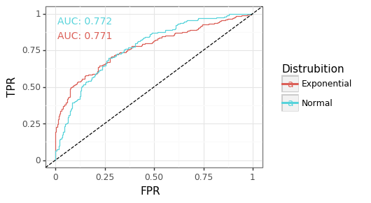
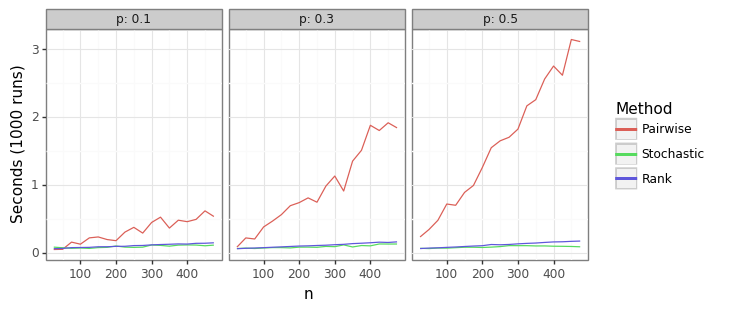
Figure 1 provides an example of two ROC curves coming from a Normal and Exponential distribution. Though the empirical AUROCs between the two curves are virtually identical, their respective sensitivity/specificity trade-offs are different. The Exponential distribution tends to have a more favourable sensitivity for high thresholds because of the right skew of the data. This figure is a reminder of some of the inherent limitations with using the AUROC as an evaluation measure. Although to repeat, the distribution of the AUROC statistic between these, or other, distributions would be the same.
The significant runtime performance gains from using the ranking approach in \eqref{eq:auc_rank} is shown in Figure 2. The pairwise method from \eqref{eq:auc_pair} is many orders of magnitude slower once the sample size is more than a few dozen observations. The stochastic method’s run time is shown to be slightly better than the ranking method. This is to be expected given that \eqref{eq:auc_rand} is linear in \(n\). However, using the stochastic approach requires picking a permutation size that leads to sufficiently tight bounds around the point estimate. The simulations below show the variation around the estimate by the number of draws.
# Get the quality of the stochastic approximation
nsim = 100
n_seq = [100, 500, 1000]
c_seq = np.arange(1,11,1).astype(int)

np.random.seed(nsim)
holder = []
for n in n_seq:
    holder_n = []
    for ii in range(nsim):
        y, s = dgp_auc(n, p, 0, dist='normal')
        gt_auc = auc_pair(y, s)
        sim_mat = np.array([[auc_rand(y, s, n*c) for c in c_seq] for x in range(nsim)])
        dat_err = np.std(gt_auc - sim_mat,axis=0)
        holder_n.append(dat_err)
    tmp = pd.DataFrame(np.array(holder_n)).melt(None,None,'c','se').assign(n=n)
    holder.append(tmp)
df_se = pd.concat(holder).reset_index(None, True)
df_se.c = df_se.c.map(dict(zip(list(range(len(c_seq))),c_seq)))
df_se = df_se.assign(sn=lambda x: pd.Categorical(x.n.astype(str),[str(z) for z in n_seq]))

plotnine.options.figure_size = (4, 3)
gg_se = (ggplot(df_se, aes(x='c',y='se',color='sn')) +
         theme_bw() + labs(y='Standard error',x='Number of draws * n') +
         geom_jitter(height=0,width=0.1,size=0.5,alpha=0.5) +
         scale_color_discrete(name='n') +
         scale_x_continuous(breaks=list(c_seq)))
gg_se
Figure 3: Variation around point estimate (stochastic)
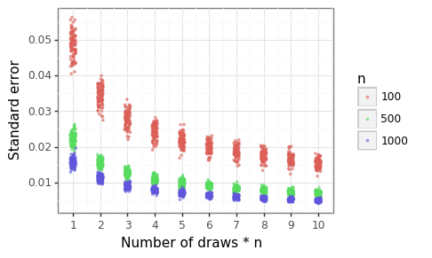
Figure 3 shows that the number of samples needed to get the standard error (SE) to ±1% for the stochastic AUROC is 4000 draws. In other words, if the actual empirical AUROC was 71%, we would expect 95% of the realizations to be around the 69-73% range for that many draws. To get to a SE of ±0.5% requires 10K draws. These results shows that unless the user is happy to tolerate an error range of more than a 0.5% percentage points, hundred of thousands of draws will be needed.
(3) Inference approaches
After reviewing the different approaches for calculating the point estimate of the empirical AUROC, attention can now be turned to doing inference on this term. Knowing that a classifier has an AUROC on 78% on a test set provides little information if there is no quantification of the uncertainty around this estimate. In this section, we’ll discuss three different approaches for generating confidence intervals (CIs). CIs are the most common method of uncertainty quantification in frequentist statistics. A two-sided CI at the \((1-\alpha)\)% level is a random variable that has the following property: \(P([l, u] \in AUC ) \geq 1-\alpha\). In other words, the probability that the true AUROC is contained within this upper and lower bound, \(l\) and \(u\) (which are random variables), is at least \((1-\alpha)\)%, meaning the true statistic of interest (the AUROC) fails to be covered by this interval at most \(\alpha\)% of the time. An exact CI will cover the true statistic of interest exactly \(1-\alpha\)% of the time, giving the test maximum power.
The approaches below are by no means exhaustive. Readers are encouraged to review other methods for other ideas.
Approach #1: Asymptotic U
As was previously mentioned, the AUROC is equivalent to an MNU test. The asymptotic properties of this statistic have been known for more than 70 years. Under the null hypothesis assumption that \(P(s_i^1 > s_i^0) = 0.5\), the asymptotic properties of the U statistic for ranks can be shown to be:
\[\begin{align*} z &= \frac{U - \mu_U}{\sigma_U} \sim N(0,1) \\ \mu_U &= \frac{n_0n_1}{2} \\ \sigma^2_U &= \frac{n_0n_1(n_0+n_1+1)}{12} \\ U &= n_1n_0 \cdot \max \{ AUC, (1-AUC) \} \\ \end{align*}\]Note that additional corrections that need to be applied in the case of data which has ties, but I will not cover this issue here. There are two clear weaknesses to this approach. First, it appeals to the asymptotic normality of the \(U\) statistic, which may be a poor approximation when \(n\) is small. Second, this formula only makes sense for testing a null hypothesis of \(AUC_0=0.5\). Notice that the constant in the denominator of the variance, 12, is the same as the constant in the variance of a uniform distribution. This is not a coincidence as the distribution of rank order statistics is uniform when the data come from the same distribution. To estimate this constant for \(AUC\neq 0.5\), Monte Carlo simulations will be needed. Specifically we want to find the right constant \(c(AUC)\) for the variance of the AUROC:
\[\begin{align*} \sigma^2_U(AUC) &= \frac{n_0n_1(n_0+n_1+1)}{c(AUC)} \end{align*}\]Even though it is somewhat computationally intensive to calculate these normalizing constants, their estimates hold true regardless of the sample of the sample sizes, as in \(c(AUC;n_0,n_1)=c(AUC;n_0’;n_1’)\) for all \(n_k, n_k’ \in \mathbb{R}^+\). The code below estimates \(c()\) and uses a spline to interpolate for values of the AUROC between the realized draws.
# PRECOMPUTE THE VARIANCE CONSTANT...
np.random.seed(1)
nsim = 10000
n1, n0 = 500, 500
den = n1 * n0
auc_seq = np.arange(0.5, 1, 0.01)
holder = np.zeros(len(auc_seq))
for i, auc in enumerate(auc_seq):
    print(i)
    mu = np.sqrt(2) * stats.norm.ppf(auc)
    Eta = np.r_[np.random.randn(n1, nsim)+mu, np.random.randn(n0,nsim)]
    Y = np.r_[np.zeros([n1,nsim],dtype=int)+1, np.zeros([n0,nsim],dtype=int)]
    R1 = stats.rankdata(Eta,axis=0)[:n1]
    Amat = (R1.sum(0) - n1*(n1+1)/2) / den
    holder[i] = (n0+n1+1) / Amat.var() / den
dat_var = pd.DataFrame({'auc':auc_seq, 'c':holder})
dat_var = pd.concat([dat_var.iloc[1:].assign(auc=lambda x: 1-x.auc), dat_var]).sort_values('auc').reset_index(None, True)
# Calculate the spline
spl = UnivariateSpline(x=dat_var.auc, y=dat_var.c)
dat_spline = pd.DataFrame({'auc':dat_var.auc, 'spline':spl(dat_var.auc)})
plotnine.options.figure_size=(4,3)
gg_c = (ggplot(dat_var,aes(x='auc',y='np.log(c)')) + theme_bw() +
        geom_point()+labs(y='log c(AUC)',x='AUROC') +
        geom_line(aes(x='auc',y='np.log(spline)'), data=dat_spline,color='red') +
       ggtitle('Red line is spline (k=3)'))
gg_c
Figure 4: Variation constant
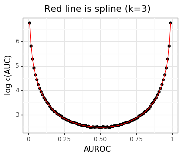
Figure 4 shows that the constant term is growing quite rapidly. The stochastic estimate of the constant at AUROC=0.5 of 11.9 is close to the true population value of 12.
Approach #2: Newcombe’s Wald Method
A second approach is to use a (relatively) new approach from Newcombe (2006). Unlike the asymptotic approach above, Newcombe’s method automatically calculates different levels of the variance for different values of the AUROC.
\[\begin{align*} \sigma^2_{AUC} &= \frac{AUC(1-AUC)}{(n_1-1)(n_0-1)} \cdot \Bigg[ 2n - 1 - \frac{3n-3}{(2-AUC)(1+AUC)} \Bigg] \end{align*}\]Assuming \(n_1 = c\cdot n\) then \(O(\sigma^2_{AUC})=\frac{AUC(1-AUC)}{n}\), which is very similar to the variance of the binomial proportion (see here).
Approach #3: Bootstrapping ranks
The final inference approach is that of the bootstrap, which generates new realizations of the statistic by resampling the data. Though the ability to get additional randomness by resampling rows of the data seems a little mysterious, if not dubious, it has a solid mathematical foundation. The bootstrap is equivalent to drawing from the empirical CDF (eCDF) of a random variable. Since the eCDF is known to be a consistent estimate of the true CDF, the error of the bootstrap will naturally decrease as \(n\) grows. The bootstrap has the attractive property that it is fully non-parametric and works well for a broad class of statistics. Note that there is no one way to do the “bootstrap” for inference, and I compare three common approaches: i) quantile, ii) classic, iii) studentized. For a review of other approaches, see here.
\[\begin{align*} \tilde{AUC}^{(k)} &= \frac{1}{n_1n_0} \sum_{i: y_i=1} \tilde{r}_i^{(k)} - \frac{n_1(n_1 +1)}{2} \\ \sigma^2_{BS} &= \frac{1}{K-1}\sum_{k=1}^K (\tilde{AUC}^{(k)} - \bar{\tilde{AUC}}) \end{align*}\]The \(k^{th}\) bootstrap (out of \(K\) total bootstraps), is generated by sampling, with replacement, the ranks of the positive score classes, and the bootstrap AUROC is calculated using the same formula from \eqref{eq:auc_rank}. Bootstrapping the ranks has the attractive property that the relative runtime is going to scale with the total number of bootstraps (\(K\)). If we had to recalculate the ranks for every bootstrap sample, then this would require an additional sorting call. The formulas for the three bootstrapping approaches are shown below for a \((1-\alpha)\)% symmetric CI.
\[\begin{align*} \text{Quantile}& \\ [l, u] &= \big[\tilde{AUC}^{(k)}_{\lfloor\alpha/2\cdot K\rfloor}, \tilde{AUC}^{(k)}_{\lceil(1-\alpha/2)\cdot K\rceil} \big] \\ \\ \text{Classic}& \\ [l, u] &= \big[AUC - \sigma_{BS}\cdot z_{1-\alpha/2}, AUC + \sigma_{BS}\cdot z_{1-\alpha/2}\big] \\ \\ \text{Studentized}& \\ [l, u] &= \big[AUC + \sigma_{BS}\cdot z_{\alpha/2}^*, AUC - \sigma_{BS}\cdot z_{1-\alpha/2}^*\big] \\ z_\alpha^* &= \Bigg[ \frac{\tilde{AUC}^{(k)} - AUC}{\sigma^{(k)}_{BS}} \Bigg]_{\lfloor\alpha\cdot K\rfloor} \end{align*}\]The quantile approach simply takes the empirical \(\alpha/2\) and \(1-\alpha/2\) quantiles of the AUROC from its bootstrapped distribution. Though the quantile approach is well suited for skewed bootstrapped distributions (i.e. the median and mean differ), it is known to be biased for small sample sizes. The classic bootstrap simply uses the empirical variance of the bootstrapped AUROCs to estimate the standard error of the statistic. Assuming that the statistic is normally distributed, the standard normal quantiles can be used to generate CIs. The Studentized approach combines the estimate of the variance from the classic bootstrap but also takes into account the possibility of skewness. For each bootstrap sample, an additional \(K\) (or some large number) bootstrapped samples are drawn, so that each bootstrapped sample has an estimate of its variance. These studentized, or normalized, scores are then used in place of the quantile from the normal distribution.
(4) Simulations
Now we are ready to test the bootstrapping methods against their analytic counterparts. The simulations below will use a 10% positive class balance, along with a range of different sample sizes. Symmetric CIs will be calculated for the 80%, 90%, and 95% level. A total of 1500 simulations are run. An 80% symmetric CI that is exact should have a coverage of 80%, meaning that the true AUROC is contained within the CIs 80% of the time. A CI that has a coverage below its nominal level will have a type-1 error rate that is greater than expected, whilst a CI that has coverage above its nominal level will have less power (i.e. a higher type-II error). In other words, the closer a CI is to its nominal level, the better.
"""
HELPER FUNCTION TO RETURN +- INTERVALS
A: array of AUCs
se: array of SEs
cv: critical values (can be array: will be treated as 1xk)
"""
def ret_lbub(A, se, cv, method):
    ub = cvec(A)+cvec(se)*rvec(cv)
    lb = cvec(A)-cvec(se)*rvec(cv)
    df_ub = pd.DataFrame(ub,columns=cn_cv).assign(bound='upper')
    df_lb = pd.DataFrame(lb,columns=cn_cv).assign(bound='lower')
    df = pd.concat([df_ub, df_lb]).assign(tt=method)
    return df

nsim = 1500
prop = 0.1
n_bs = 1000
n_student = 250
n_seq = [50, 100, 250, 1000]#[]
auc_seq = [0.5, 0.7, 0.9 ]  #"true" AUROC between the distributions
pvals = (1-np.array([0.8, 0.9, 0.95]))/2
crit_vals = np.abs(stats.norm.ppf(pvals))
cn_cv = ['p'+str(i+1) for i in range(len(pvals))]

np.random.seed(1)

holder = []
for n in n_seq:
    for auc in auc_seq:
        print('n: %i, AUROC: %0.2f' % (n, auc))
        n1 = int(np.round(n * prop))
        n0 = n - n1
        den = n1*n0
        mu = np.sqrt(2) * stats.norm.ppf(auc)
        Eta = np.r_[np.random.randn(n1, nsim)+mu, np.random.randn(n0,nsim)]
        Y = np.r_[np.zeros([n1,nsim],dtype=int)+1, np.zeros([n0,nsim],dtype=int)]
        # Calculate the AUCs across the columns
        R1 = stats.rankdata(Eta,axis=0)[:n1]
        Amat = (R1.sum(0) - n1*(n1+1)/2) / den
        # --- Approach 1: Asymptotic U --- #
        sd_u = np.sqrt((n0+n1+1)/spl(Amat)/den)
        df_asym = ret_lbub(Amat, sd_u, crit_vals, 'asymptotic')
        # --- Approach 2: Newcombe's wald
        sd_newcombe = np.sqrt(Amat*(1-Amat)/((n1-1)*(n0-1))*(2*n-1-((3*n-3)/((2-Amat)*(1+Amat)))))
        df_newcombe = ret_lbub(Amat, sd_newcombe, crit_vals, 'newcombe')
        # --- Approach 3: Bootstrap the ranks --- #
        R1_bs = pd.DataFrame(R1).sample(frac=n_bs,replace=True).values.reshape([n_bs]+list(R1.shape))
        auc_bs = (R1_bs.sum(1) - n1*(n1+1)/2) / den
        sd_bs = auc_bs.std(0,ddof=1)
        # - (i) Standard error method - #
        df_bs_se = ret_lbub(Amat, sd_bs, crit_vals, 'bootstrap_se')
        # - (ii) Quantile method - #
        df_lb_bs = pd.DataFrame(np.quantile(auc_bs,pvals,axis=0).T,columns=cn_cv).assign(bound='lower')
        df_ub_bs = pd.DataFrame(np.quantile(auc_bs,1-pvals,axis=0).T,columns=cn_cv).assign(bound='upper')
        df_bs_q = pd.concat([df_ub_bs, df_lb_bs]).assign(tt='bootstrap_q')
        # - (iii) Studentized - #
        se_bs_s = np.zeros(auc_bs.shape)
        for j in range(n_bs):
            R1_bs_s = pd.DataFrame(R1_bs[j]).sample(frac=n_student,replace=True).values.reshape([n_student]+list(R1.shape))
            auc_bs_s = (R1_bs_s.sum(1) - n1*(n1+1)/2) / den
            se_bs_s[j] = auc_bs_s.std(0,ddof=1)
        # Get the t-score dist
        t_bs = (auc_bs - rvec(Amat))/se_bs_s
        df_lb_t = pd.DataFrame(cvec(Amat) - cvec(sd_bs)*np.quantile(t_bs,1-pvals,axis=0).T,columns=cn_cv).assign(bound='lower')
        df_ub_t = pd.DataFrame(cvec(Amat) - cvec(sd_bs)*np.quantile(t_bs,pvals,axis=0).T,columns=cn_cv).assign(bound='upper')
        df_t = pd.concat([df_ub_t, df_lb_t]).assign(tt='bootstrap_s')
        # Combine
        tmp_sim = pd.concat([df_asym, df_newcombe, df_bs_se, df_bs_q, df_t]).assign(auc=auc, n=n)
        holder.append(tmp_sim)
# Merge and save
res = pd.concat(holder)
res = res.rename_axis('idx').reset_index().melt(['idx','bound','tt','auc','n'],cn_cv,'tpr')
res = res.pivot_table('value',['idx','tt','auc','n','tpr'],'bound').reset_index()
res.tpr = res.tpr.map(dict(zip(cn_cv, 1-2*pvals)))
res = res.assign(is_covered=lambda x: (x.lower <= x.auc) & (x.upper >= x.auc))
res_cov = res.groupby(['tt','auc','n','tpr']).is_covered.mean().reset_index()
res_cov = res_cov.assign(sn = lambda x: pd.Categorical(x.n, x.n.unique()))
lvls_approach = ['asymptotic','newcombe','bootstrap_q','bootstrap_se','bootstrap_s']
lbls_approach = ['Asymptotic', 'Newcombe', 'BS (Quantile)', 'BS (Classic)', 'BS (Studentized)']
res_cov = res_cov.assign(tt = lambda x: pd.Categorical(x.tt, lvls_approach).map(dict(zip(lvls_approach, lbls_approach))))
res_cov.rename(columns={'tpr':'CoverageTarget', 'auc':'AUROC'}, inplace=True)

tmp = pd.DataFrame({'CoverageTarget':1-2*pvals, 'ybar':1-2*pvals})
plotnine.options.figure_size = (6.5, 5)
gg_cov = (ggplot(res_cov, aes(x='tt', y='is_covered',color='sn')) +
         theme_bw() + geom_point() +
         facet_grid('AUROC~CoverageTarget',labeller=label_both) +
         theme(axis_text_x=element_text(angle=90), axis_title_x=element_blank()) +
         labs(y='Coverage') +
         geom_hline(aes(yintercept='ybar'),data=tmp) +
         scale_color_discrete(name='Sample size'))
gg_cov
Figure 5: Coverage results by method
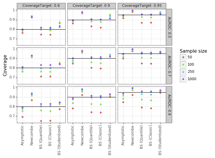
Figure 5 shows the coverage results for the different approaches across different conditions. Newcombe’s method is consistently the worst performer, with the CIs being much too conservative. The estimated SEs are at least 40% larger than the asymptotic ones (code not shown), leading to a CI with significantly reduced power. The asymptotic approach and quantile/classic bootstrap have SEs which are too small when the sample size is limited, leading to under-coverage and an inflated type-I error rate. Once the sample size reaches 1000, the asymptotic intervals are quite accurate. The studentized bootstrap is the most consistently accurate approach, especially for small sample sizes, and tends to be conservative (over-coverage). Overall the studentized bootstrap is the clear winner. However, it is also the most computationally costly, which means for large samples the asymptotic estimates may be better.
(5) Ranking bootstraps?
Readers may be curious whether ranking the bootstraps, rather than bootstrapping the ranks, may lead to better inference. Section (3) has already noted the obvious computational gains from bootstrapping the ranks. Despite my initial assumption that ranking the bootstraps would lead to more variation because of the additional randomness in the negative class, this turned out not to be the case due to the creation of ties in the scores which reduces the variation in the final AUROC estimate. The simulation block shows that the SE of the bootstrapped ranks is higher than the ranked bootstraps in terms of the AUROC statistic. Since the bootstrap approaches did not generally have a problem of over-coverage, the smaller SEs will lead to higher type-I error rates, especially for small sample sizes. In this case, the statistical advantages of bootstrapping the ranks also coincide with a computational benefit.
seed = 1
np.random.seed(seed)
n_bs, nsim = 1000, 1500
n1, n0, mu = 25, 75, 1
s = np.concatenate((np.random.randn(n1, nsim)+mu, np.random.randn(n0,nsim)))
y = np.concatenate((np.repeat(1,n1),np.repeat(0,n0)))
r = stats.rankdata(s,axis=0)[:n1]
s1, s0 = s[:n1], s[n1:]
r_bs = pd.DataFrame(r).sample(frac=n_bs,replace=True,random_state=seed).values.reshape([n_bs]+list(r.shape))
s_bs1 = pd.DataFrame(s1).sample(frac=n_bs,replace=True,random_state=seed).values.reshape([n_bs]+list(s1.shape))
s_bs0 = pd.DataFrame(s0).sample(frac=n_bs,replace=True,random_state=seed).values.reshape([n_bs]+list(s0.shape))
s_bs = np.concatenate((s_bs1, s_bs0),axis=1)
r_s_bs = stats.rankdata(s_bs,axis=1)[:,:n1,:]
auc_bs = (r_bs.sum(1) - n1*(n1+1)/2)/(n1*n0)
auc_s_bs = (r_s_bs.sum(1) - n1*(n1+1)/2)/(n1*n0)
se_bs = auc_bs.std(0)
se_s_bs = auc_s_bs.std(0)
df_bs = pd.DataFrame({'bs_r':se_bs, 'r_bs':se_s_bs})
print('Mean AUROC for bootstrapping ranks: %0.3f, and ranking bootstraps: %0.3f' %
      (np.mean(df_bs.bs_r),np.mean(df_bs.r_bs)))
Mean AUROC for bootstrapping ranks: 0.064, and ranking bootstraps: 0.054