
Direct AUROC optimization with PyTorch
\(\newcommand{\by}{\boldsymbol{y}}\) \(\newcommand{\beta}{\boldsymbol{\eta}}\) \(\newcommand{\bw}{\boldsymbol{w}}\) \(\newcommand{\bx}{\boldsymbol{x}}\)
In this post I’ll discuss how to directly optimize the Area Under the Receiver Operating Characteristic Curve (AUROC), which measures the discriminatory ability of a model across a range of sensitivity and specificity thresholds for binary classification. The AUROC is often used as method to benchmark different models and has the added benefit that its properties are independent of the underlying class imbalance.
The AUROC is a specific instance of the more general learning to rank class of problems as the AUROC is the proportion of scores from a positive class that exceed the scores from a negative class. More formally if the outcome for the \(i^{th}\) observation is \(y \in \{0,1\}\) and has a corresponding risk score \(\eta_i\), then the AUROC for \(\by\) and \(\beta\) will be:
\[\begin{align*} \text{AUROC}(\by,\beta) &= \frac{1}{|I_1|\cdot|I_0|} \sum_{i \in I_1} \sum_{j \in I_0} \Big[ I[\eta_i > \eta_j] + 0.5I[\eta_i = \eta_j] \Big] \\ I_k &= \{i: y_i = k \} \end{align*}\]Most AUROC formulas grant a half-point for tied scores. As has been discussed before, optimizing indicator functions \(I(\cdot)\) is NP-hard, so instead a convex relation of the AUROC can be calculated.
\[\begin{align*} \text{cAUROC}(\by,\beta) &= \frac{1}{|I_1|\cdot|I_0|} \sum_{i \in I_1} \sum_{j \in I_0} \log \sigma [\eta_i - \eta_j] \\ \sigma(z) &= \frac{1}{1+\exp(-z)} \end{align*}\]The cAUROC formula encourages the log-odds of the positive class (\(y=1\)) to be as large as possible with respect to the negative class (\(y=0\)).
(1) Optimization with linear methods
Before looking at a neural network method, this first section will show how to directly optimize the cAUROC with a linear combination of features. This approach will be compared to the standard logistic regression method to see if there is a meaningful difference. By encoding \(\eta_i = \bx_i^T\bw\) as linear in the feature space and applying the chain rule, the derivative of the cAUROC with respect to the weights is:
\[\begin{align*} \frac{\partial \text{cAUROC}(\by,\beta)}{\partial \bw} &= \frac{1}{|I_1|\cdot|I_0|} \sum_{i \in I_1} \sum_{j \in I_0} (1 - \sigma [\eta_i - \eta_j] ) [\bx_i - \bx_j] \end{align*}\]# Import the necessary modules
import numpy as np
from scipy.optimize import minimize
def sigmoid(x):
return( 1 / (1 + np.exp(-x)) )
def idx_I0I1(y):
return( (np.where(y == 0)[0], np.where(y == 1)[0] ) )
def AUROC(eta,idx0,idx1):
den = len(idx0) * len(idx1)
num = 0
for i in idx1:
num += sum( eta[i] > eta[idx0] ) + 0.5*sum(eta[i] == eta[idx0])
return(num / den)
def cAUROC(w,X,idx0,idx1):
eta = X.dot(w)
den = len(idx0) * len(idx1)
num = 0
for i in idx1:
num += sum( np.log(sigmoid(eta[i] - eta[idx0])) )
return( - num / den)
def dcAUROC(w, X, idx0, idx1):
eta = X.dot(w)
n0, n1 = len(idx0), len(idx1)
den = n0 * n1
num = 0
for i in idx1:
num += ((1 - sigmoid(eta[i] - eta[idx0])).reshape([n0,1]) * (X[[i]] - X[idx0]) ).sum(axis=0) # *
return( - num / den)
In the example simulations below the Boston dataset will be used where the binary outcome is whether a house price is in the 90th percentile or higher (i.e. the top 10% of prices in the distribution).
import pandas as pd
from sklearn.datasets import load_boston
from sklearn.linear_model import LogisticRegression
from sklearn.metrics import roc_auc_score
from sklearn.model_selection import train_test_split
from sklearn.preprocessing import StandardScaler
X, y = load_boston(return_X_y=True)
# binarize
y = np.where(y > np.quantile(y,0.9), 1 , 0)

nsim = 100
holder_auc = []
holder_w = []
winit = np.repeat(0,X.shape[1])
for kk in range(nsim):
  y_train, y_test, X_train, X_test = train_test_split(y, X, test_size=0.2, random_state=kk, stratify=y)
  enc = StandardScaler().fit(X_train)
  idx0_train, idx1_train = idx_I0I1(y_train)
  idx0_test, idx1_test = idx_I0I1(y_test)
  w_auc = minimize(fun=cAUROC,x0=winit,
                  args=(enc.transform(X_train), idx0_train, idx1_train),
                  method='L-BFGS-B',jac=dcAUROC).x
  eta_auc = enc.transform(X_test).dot(w_auc)
  mdl_logit = LogisticRegression(penalty='none')
  eta_logit = mdl_logit.fit(enc.transform(X_train),y_train).predict_proba(X_test)[:,1]
  auc1, auc2 = roc_auc_score(y_test,eta_auc), roc_auc_score(y_test,eta_logit)
  holder_auc.append([auc1, auc2])
  holder_w.append(pd.DataFrame({'cn':load_boston()['feature_names'],'auc':w_auc,'logit':mdl_logit.coef_.flatten()}))

auc_mu = np.vstack(holder_auc).mean(axis=0)
print('AUC from cAUROC: %0.2f%%\nAUC for LogisticRegression: %0.2f%%' %
      (auc_mu[0], auc_mu[1]))
AUC from cAUROC: 0.96%
AUC for LogisticRegression: 0.69%
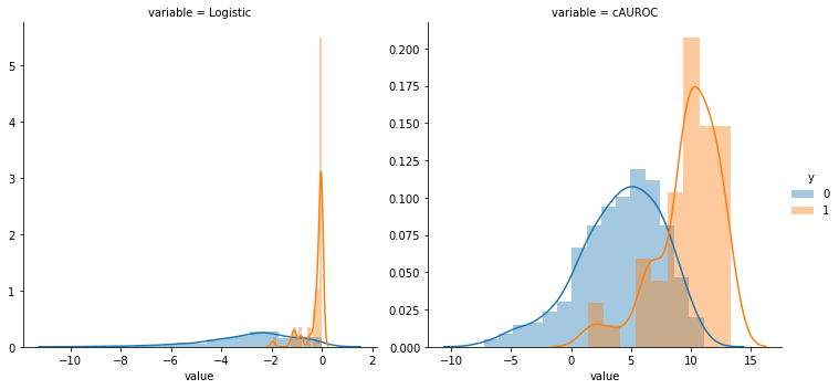
The cAUROC maximizer finds a linear combination of features that has a significantly higher AUROC when compared to logistic regression. This is to be expected in cases with a strong class imbalance as the logistic loss will incentivize the model gradients towards weights that achieve low predicted probabilities because most of the labels are zero (or one). In contrast, the cAUROC maximizer is independent of any class imbalance and therefore does not suffer from this bias. The figure below shows the relative overlap between the two distributions generated by each linear model on the entire dataset. The cAUROC model has a smoother relationship and is less prone to overfitting.
enc = StandardScaler().fit(X)
idx0, idx1 = idx_I0I1(y)
w_auc = minimize(fun=cAUROC,x0=winit,args=(enc.transform(X), idx0, idx1),
                method='L-BFGS-B',jac=dcAUROC).x
eta_auc = enc.transform(enc.transform(X)).dot(w_auc)
eta_logit = LogisticRegression(max_iter=1e3).fit(enc.transform(enc.transform(X)),
                        y).predict_log_proba(enc.transform(X))[:,1]

tmp = pd.DataFrame({'y':y,'Logistic':eta_logit,'cAUROC':eta_auc}).melt('y')
g = sns.FacetGrid(data=tmp,hue='y',col='variable',sharex=False,sharey=False,height=5)
g.map(sns.distplot,'value')
g.add_legend()
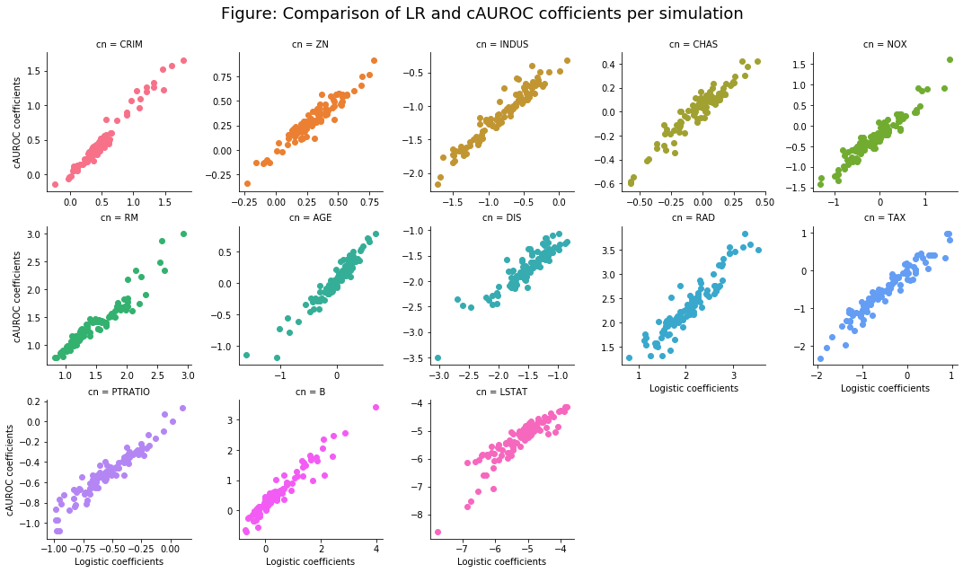
The figure below shows that while the coefficients between the cAUROC model and logistic regression are highly correlated, their slight differences still lead to meaningful out-of-sample performance gains.
import seaborn as sns
from matplotlib import pyplot as plt

df_w = pd.concat(holder_w) #.groupby('cn').mean().reset_index()
g = sns.FacetGrid(data=df_w,col='cn',col_wrap=5,hue='cn',sharex=False,sharey=False)
g.map(plt.scatter, 'logit','auc')
g.set_xlabels('Logistic coefficients')
g.set_ylabels('cAUROC coefficients')
plt.subplots_adjust(top=0.9)
g.fig.suptitle('Figure: Comparison of LR and cAUROC cofficients per simulation',fontsize=18)
(2) AUROC maximization with PyTorch
To optimize a neural network in PyTorch with the goal of maximizing the cAUROC we will draw a given \(i,j\) pair where \(i \in I_1\) and \(j \in I_0\). While other mini-batch approaches are possible (including the full-batch approach used for the gradient functions above), using a mini-batch of two will have the smallest memory overhead. The stochastic gradient for our network \(f_\theta\) will now be:
\[\begin{align*} \Bigg[\frac{\partial f_\theta}{\partial \theta}\Bigg]_{i,j} &= \frac{\partial}{\partial \theta} \log \sigma [ f_\theta(\bx_i) - f_\theta(\bx_j) ] \end{align*}\]Where \(f(\cdot)\) is the output from the neural network and \(\theta\) are the network parameters. The gradient of this deep neural network will be calculated by PyTorch’s automatic differention backend.
The example dataset will be the California housing price dataset. To make the prediction task more challenging, house prices will first be partially scrambled with noise, and then the outcome will binarized by labeling only the top 5% of housing prices as the positive class.
from sklearn.datasets import fetch_california_housing

np.random.seed(1234)
data = fetch_california_housing(download_if_missing=True)
cn_cali = data.feature_names
X_cali = data.data
y_cali = data.target
y_cali += np.random.randn(y_cali.shape[0])*(y_cali.std())
y_cali = np.where(y_cali > np.quantile(y_cali,0.95),1,0)
y_cali_train, y_cali_test, X_cali_train, X_cali_test = \
  train_test_split(y_cali, X_cali, test_size=0.2, random_state=1234, stratify=y_cali)
enc = StandardScaler().fit(X_cali_train)
The code block below defines the neural network class, optimizer, and loss function.
import torch
import torch.nn as nn
import torch.nn.functional as F

class ffnet(nn.Module):
    def __init__(self,num_features):
      super(ffnet, self).__init__()
      p = num_features
      self.fc1 = nn.Linear(p, 36)
      self.fc2 = nn.Linear(36, 12)
      self.fc3 = nn.Linear(12, 6)
      self.fc4 = nn.Linear(6,1)

    def forward(self,x):
      x = F.relu(self.fc1(x))
      x = F.relu(self.fc2(x))
      x = F.relu(self.fc3(x))
      x = self.fc4(x)
      return(x)

# Binary loss function
criterion = nn.BCEWithLogitsLoss()
# Seed the network
torch.manual_seed(1234)
nnet = ffnet(num_features=X_cali.shape[1])
optimizer = torch.optim.Adam(params=nnet.parameters(),lr=0.001)
In the next code block, we’ll set up the sampling strategy and train the network until the AUC exceeds 90% on the validation set, at which point training will be terminated.
np.random.seed(1234)

y_cali_R, y_cali_V, X_cali_R, X_cali_V = \
  train_test_split(y_cali_train, X_cali_train, test_size=0.2, random_state=1234, stratify=y_cali_train)
enc = StandardScaler().fit(X_cali_R)

idx0_R, idx1_R = idx_I0I1(y_cali_R)

nepochs = 100

auc_holder = []
for kk in range(nepochs):
  print('Epoch %i of %i' % (kk+1, nepochs))
  # Sample class 0 pairs
  idx0_kk = np.random.choice(idx0_R,len(idx1_R),replace=False)
  for i,j in zip(idx1_R, idx0_kk):
    optimizer.zero_grad() # clear gradient
    dlogit = nnet(torch.Tensor(enc.transform(X_cali_R[[i]]))) - \
        nnet(torch.Tensor(enc.transform(X_cali_R[[j]]))) # calculate log-odd differences
    loss = criterion(dlogit.flatten(), torch.Tensor([1]))
    loss.backward() # backprop
    optimizer.step() # gradient-step
  # Calculate AUC on held-out validation
  auc_k = roc_auc_score(y_cali_V,
    nnet(torch.Tensor(enc.transform(X_cali_V))).detach().flatten().numpy())
  if auc_k > 0.9:
    print('AUC > 90% achieved')
    break
Epoch 1 of 100
Epoch 2 of 100
Epoch 3 of 100
Epoch 4 of 100
Epoch 5 of 100
Epoch 6 of 100
Epoch 7 of 100
Epoch 8 of 100
Epoch 9 of 100
Epoch 10 of 100
Epoch 11 of 100
Epoch 12 of 100
Epoch 13 of 100
AUC > 90% achieved
# Compare performance on final test set
auc_nnet_cali = roc_auc_score(y_cali_test,
    nnet(torch.Tensor(enc.transform(X_cali_test))).detach().flatten().numpy())

# Fit a benchmark model
logit_cali = LogisticRegression(penalty='none',solver='lbfgs',max_iter=1000)
logit_cali.fit(enc.transform(X_cali_train), y_cali_train)
auc_logit_cali = roc_auc_score(y_cali_test,logit_cali.predict_proba(enc.transform(X_cali_test))[:,1])

print('nnet-AUC: %0.3f, logit: %0.3f' % (auc_nnet_cali, auc_logit_cali))
nnet-AUC: 0.894, logit: 0.873
While the gain in performance has turned out to be minimal for this dataset (an extra 2% AUROC), the exercise has nevertheless revealed how easy it is to write an optimizer in PyTorch for a neural network architecture to achieve direct AUROC maximization. Specifically, learn-to-rank architectures can be carried out by re-purposing the cross entropy loss (e.g BCEWithLogitsLoss) to encourage the model to find a parameterization which gets the pairwise ordering correct.