Introduction

In the binary classification setting linear models such as logistic regression, suport vector machines, and the linear discriminant analyis are often used when a researcher is interested in obtaining a simple model that can be fit quickly and returns interpretable results. These linear models models can also be combined with regularization techniques that allow for a better balancing of the bias-variance trade-off and can incorporate known structural features of the data. However the loss functions that are usually used to train these models can be poor surrogates for the desired performance metrics. For example in biomedical research the AUC, or area under the ROC curve, is often the preferred evaluation metric because it both summarizes the sensitivity and specificity of a classifier and avoids some of the issues stemming from class imbalances (i.e. a large ratio of positive to negative class labels or vice versa).[¹] The AUC of a model can be interpreted as the probability that the score generated by that model for a positive class label will exceed the score generated by that model for a negative class.[²] In this post I will review an interesting optimization technique developed by Ghanbari and Scheinberg in their recent arXiv paper Directly and Efficiently Optimizing Prediction Error and AUC of Linear Classifiers. While their paper focuses on the mathematical details, I will show how to implement this approach in R.

The notation used in this post is as follows: assume some machine learning model maps a \(p\)-dimensional feature vector \(\xb\) to a real number, \(f(\xb,\thetab): \mathbb{R}^p \to \mathbb{R}\), where \(\theta\) is some learned parameter over \(n\) sample tuples of the training data \((\xbi,y_i)\) with a binary response \(y=\pm1\). The feature map will be assumed to be linear (this turns out to be a critical assumption): \(f(\xb,\thetab) = \xb^T\thetab\).

The formal of the AUC loss of a linear classifier and its risk are shown below.

In other words the risk shown in \eqref{eq:auc_risk} (the expected value of our loss function) is the probability that the risk score of the positive class will exceed that of a negative class. This definition reveals why the given dataset class imbalances do not factor into the loss metric.

Mixture of Gaussians formulation

The second key assumption (in addition to linearity) is that that the distribution of the design matrix comes from two different conditional Gaussian distributions. The Gaussian distribution has the nice property that linear combinations of a Gaussian random vector/variable will remain Gaussian as well as vector concatenations.

Next consider the following univariate Gaussian random variable.

Notice that the random variable \(Z_\thetab\) in \eqref{eq:varz} matches term seem in the AUC risk from \eqref{eq:auc_risk} and that we can set \(\Sigmab^-_+=\boldsymbol{0}\) since the two random variables are independent of each other. Hence if we want to maximize the AUC, we only have to maximize the parameter vector inside a Gaussian normal CDF \(\Phi\).

The gradient of the loss function \eqref{eq:loss} can be found by using Leibniz’s differentian rule.

The loss function \eqref{eq:loss} is trying to find a vector \(\thetab\) that leads to a mean as many standard deviations from zero as possible. Note that function is not evaluable when \(\thetab=\boldsymbol{0}\).

Code Implementation

As the relevant loss function and gradient for the Gaussian-AUC optimization only require the pre-computed \(\mub\) and \(\Sigmab\), their optimization is straight-forward.

Loss function \(\ell(\thetab)\) from \eqref{eq:loss}

lfun.auc <- function(theta,mu,Sigma) {
  mu.theta <- sum( theta * mu )
  mu.Sigma2 <- as.numeric( t(theta) %*% Sigma %*% theta )
  mu.Sigma <- sqrt(mu.Sigma2)
  score <- -1 * pnorm(q=mu.theta/mu.Sigma)
  return(score)
}

Gradient of loss \(\nabla_\theta \ell(\thetab)\) from \eqref{eq:grad}

gfun.auc <- function(theta, mu, Sigma) {
  mu.theta <- sum( theta * mu )
  gtheta <- Sigma %*% theta
  mu.Sigma2 <- as.numeric( t(theta) %*%  gtheta )
  mu.Sigma <- sqrt(mu.Sigma2)
  grad <- -1/sqrt(2*pi) * exp(-0.5 * (mu.theta / mu.Sigma)^2 ) * ( mu.Sigma*mu - (mu.theta/mu.Sigma)*as.vector(gtheta) )/mu.Sigma^2
  return(grad)
}

Wrapper (uses base optim function)

auc.optim <- function(X, y, theta_init=NULL, standardize=TRUE) {
  y <- ifelse(y == 0,-1,1)
  stopifnot(all(y %in% c(1,-1)))
  stopifnot(is.matrix(X))
  idx.p <- which(y == +1)
  idx.n <- which(y == -1)
  if (standardize) {
    X <- scale(X)
    X.sd <- attr(X,'scaled:scale')
  } else {
    X.sd <- rep(1,ncol(X))
  }
  mu <- apply(X[y==+1,],2,mean) - apply(X[y==-1,],2,mean)
  Sigma <- cov(X[y==+1,]) + cov(X[y==-1,])
  if (is.null(theta_init)) { theta_init = mu }
  tmp.fit <- optim(par=theta_init, fn=lfun.auc, gr=gfun.auc, mu=mu, Sigma=Sigma, method = 'BFGS')
  theta_hat <- tmp.fit$par/X.sd
  return(theta_hat)
}

While \eqref{eq:loss} is not convex per se, many of its local minima turn out to be multiple global minima as well. This is because if \(\hat{\thetab}_A\) achieve some loss \(\ell_A\), then \(\hat{\thetab}_B=c\cdot \hat{\thetab}_A\) where \(c>0\) will obtain the same loss since the order of risk scores will remain unchanged. This property can be observed by initializing the algorithm at different starting values and noticing that while they return different \(\hat{\thetab}\)’s, they all have the same loss and ratio of \(\hat{\thetab}_1 / \hat{\thetab}_2\).

Example with the iris dataset

To build some intuition for how this approach works consider drawing a decision line that will achieve the highest AUC when classifying the versicolor and virginica flowers in the iris data using the first two features (Sepal.Length and Sepal.Width). The figure below shows the linear decision boundary that a logistic regression classifier would obtain. Notice that regardless of how the line is drawn, the AUC will be less than 100%.

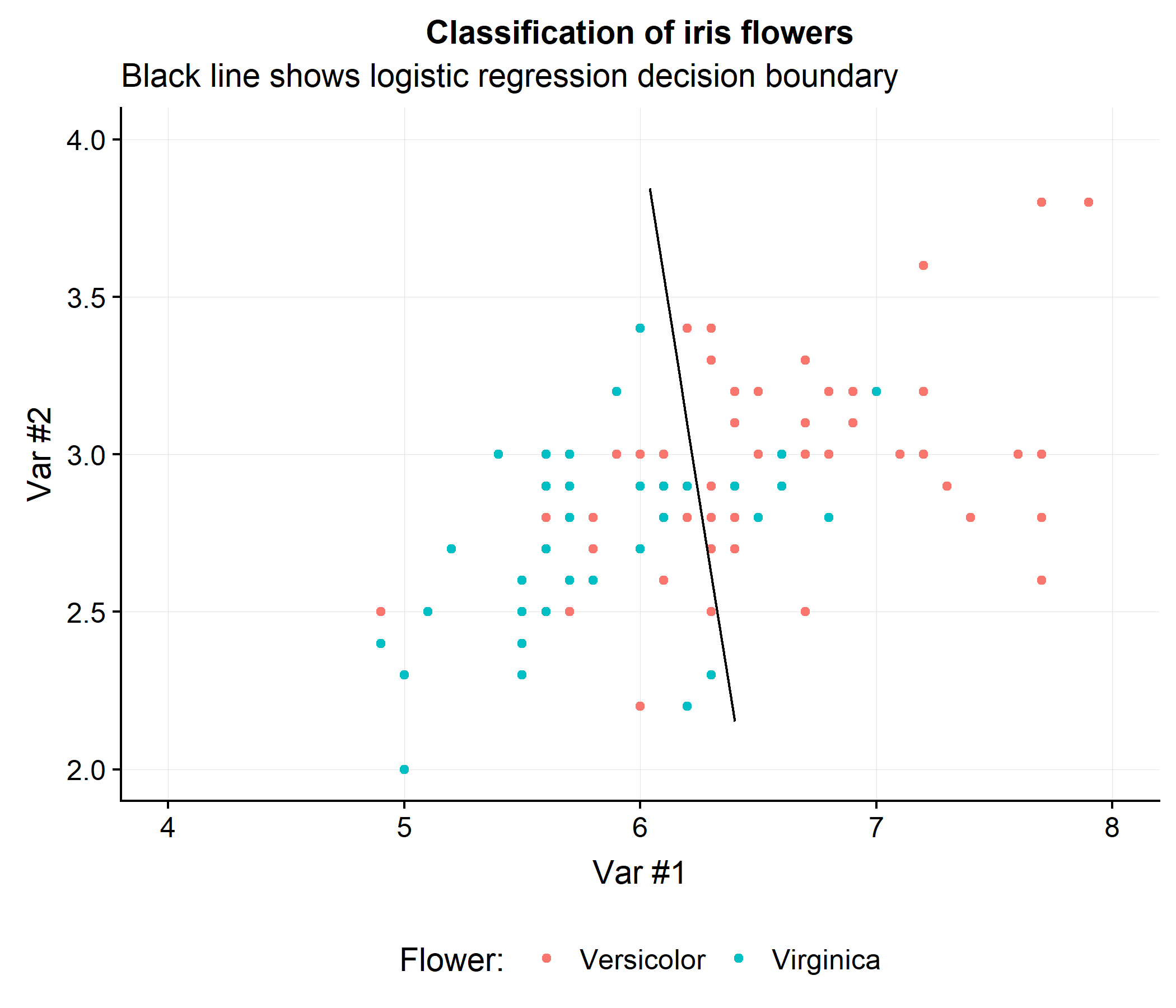
While a perfect AUC is not possible, does this linear decision boundary necessary optimize the AUC? Let’s look at the performance of this classifier.

dat <- iris[iris$Species != 'setosa',]
y <- ifelse(dat$Species=='versicolor',1,0)
X <- as.matrix(dat[,1:2])
mdl.logistic <- glm(y ~ X, family=binomial)
 
auc.function <- auc.fun <- function(y,rsk) {
  idx1 <- which( y == 1 )
  idx0 <- which( y == 0 )
  rsk1 <- rsk[idx1]
  rsk0 <- rsk[idx0]
  num <- 0
  den <- 0
  for (i in seq_along(rsk1)) {
    comp <- rsk1[i] > rsk0
    num <- num + sum(comp)
    den <- den + length(comp)
  }
  auc <- num / den
  return(auc)
}
print(sprintf('AUC of logistic classifier: %0.3f',auc.function(y=y, rsk=predict(mdl.logistic))))

## [1] "AUC of logistic classifier: 0.789"

Which turns out to be virtually the same as the Gaussian-AUC approach.

print(sprintf('AUC of Gaussian-AUC classifier: %0.3f',auc.function(y=y, rsk=X %*% auc.optim(X,y))))

## [1] "AUC of Gaussian-AUC classifier: 0.789"

However the Gaussian-AUC method does slightly better in the leave-one-out setting.

rsk_logit_loo <- sapply(seq(nrow(X)),function(ii) sum(glm(y[-ii] ~ X[-ii,],family=binomial)$coef * c(1,X[ii,])) )
rsk_auc_loo <- sapply(seq(nrow(X)),function(ii) sum(X[ii,] * auc.optim(X[-ii,],y[-ii])) )
print(sprintf('AUC from Gaussian-AUC: %0.3f and Logistic: %0.3f',auc.fun(y=y, rsk=rsk_auc_loo),auc.fun(y=y, rsk=rsk_logit_loo)))

## [1] "AUC from Gaussian-AUC: 0.772 and Logistic: 0.768"

Concluding thoughts

The Gaussian-AUC approach has several noticeable advantages. First, it scales incredibly well as \(n\) grows, since the calculation of \(\mub\) and \(\Sigmab\) can be done in a single pass and then the data can be discarded. Second, the optimization procedure is very simple and can be solved with simple first- or second-order methods (in this post the quasi-Newton BFGS algorithm was used). This loss function could also be incorporated into more complex models such a feed-forward Neural networks, with an additional loss likely needed to ensure the output layers have a conditional Gaussian distribution. In the case of survival modelling, it would be easy to approximate the time-dependent AUC loss function by using multiple mean and variance terms for each time point under evaluation.

However this approach has two key limiting factors. First, for high-dimensional datasets, the estimate of \(\Sigmab\) will become non-identifiable when \(p \gg n\) and the high-dimensional covariance matrix will need to be estimated with regularized techniques like the Graphical Lasso. An associated issue is that the memory cost of storing and evaluating \(\thetab^T \Sigmab\) will become prohibitive for large \(p\) as well. Second, because the approach is a non-convex optimization problem, the inclusion of regularization forces to the coefficients to zero very quickly. This is in contrast to other non-convex problems where regularization actually helps! Despite these drawbacks, the Gaussian-AUC approach is a useful and fast method for obtaining linear decision boundaries which directly optimize an AUC surrogate and work well in the \(n \gg p\) environment.