Over the last fifteen years the field of biology has undergone a significant cultural change. The pipette is being replaced by the piping operator. At the recent Software Carpentry workshop that occurred at Queen’s University this week, I noticed that most of the people there to learn about UNIX programming were biologists[¹]. As the cost of high-throughput sequencing technology has fallen, the possibility of extracting important patterns, or biomarkers, from these high-dimensional data sets has increased. However, the need for robust statistical procedures for understanding and mining these data sets remains more important than ever. This post will use a machine learning approach for estimating classification accuracy in a small \(N\) large \(p\) environment, using data from an interesting 2012 paper, Epigenetic markers of prostate cancer in plasma circulating DNA by Cortese et al. (2012). The goal of this post will be twofold: (1) outline the theoretical challenges in approximating out-of-sample accuracy in small \(N\) large \(p\) environments, and (2) construct a machine learning pipeline that determines the best model for cancer classification using a cirDNA data set with 4000+ features and only 39 observations.

Introduction and data exploration

In Cortese et al. (2012) the researchers were interested in whether modifications to circulating DNA (cirDNA) contained biomarkers for prostate cancer patients. Were such patterns to exist, a non-invasive biomarker could potentially be used for assessing prostate cancer risk. The paper took a multi-faceted approach and had several findings:

1. DNA modification to regions adjacent to the gene encoding ring finger protein 219 distinguished prostate cancer from benign hyperplasias with good sensitivity (61%) and specificity (71%).
2. Repetitive sequences indicated a highly statistically significant loss of DNA at the pericentromeric region of chromosome 10 in prostate cancer patients.
3. A machine-learning technique developed using multi-locus biomarkers was able to correctly distinguished prostate cancer samples from unaffected controls with 72% accuracy.

The last finding of the paper is of interest to this post. However, we will begin with an exploration of the data. One of the nice things about the field of genomics is that data used in academic papers is usually posted on the NCBI’s GEO, with this study being no exception. Here is a quick overview of the steps used to bring in and tidy the data.

1. The .gpr files were loaded using the read.maimages, backgroundCorrect, and normalizeWithinArrays functions from the limma package in R. The last function generates a red/green intensity ratio (log base 2). The two replicates were then averaged per probe.
2. The microarray data was generated from a “UHN Human CpG 12K Array”, and annotation data was downloadable from the NCBI site. Annotation data was matched to TxDb.Hsapiens.UCSC.hg19.knownGene from the Homo.sapiens package by finding common overlap in DNA sequences. Where matching was not perfect, the closest gene location was used.
3. Duplicate and unknown genes were dropped. This left more than 4200 features.

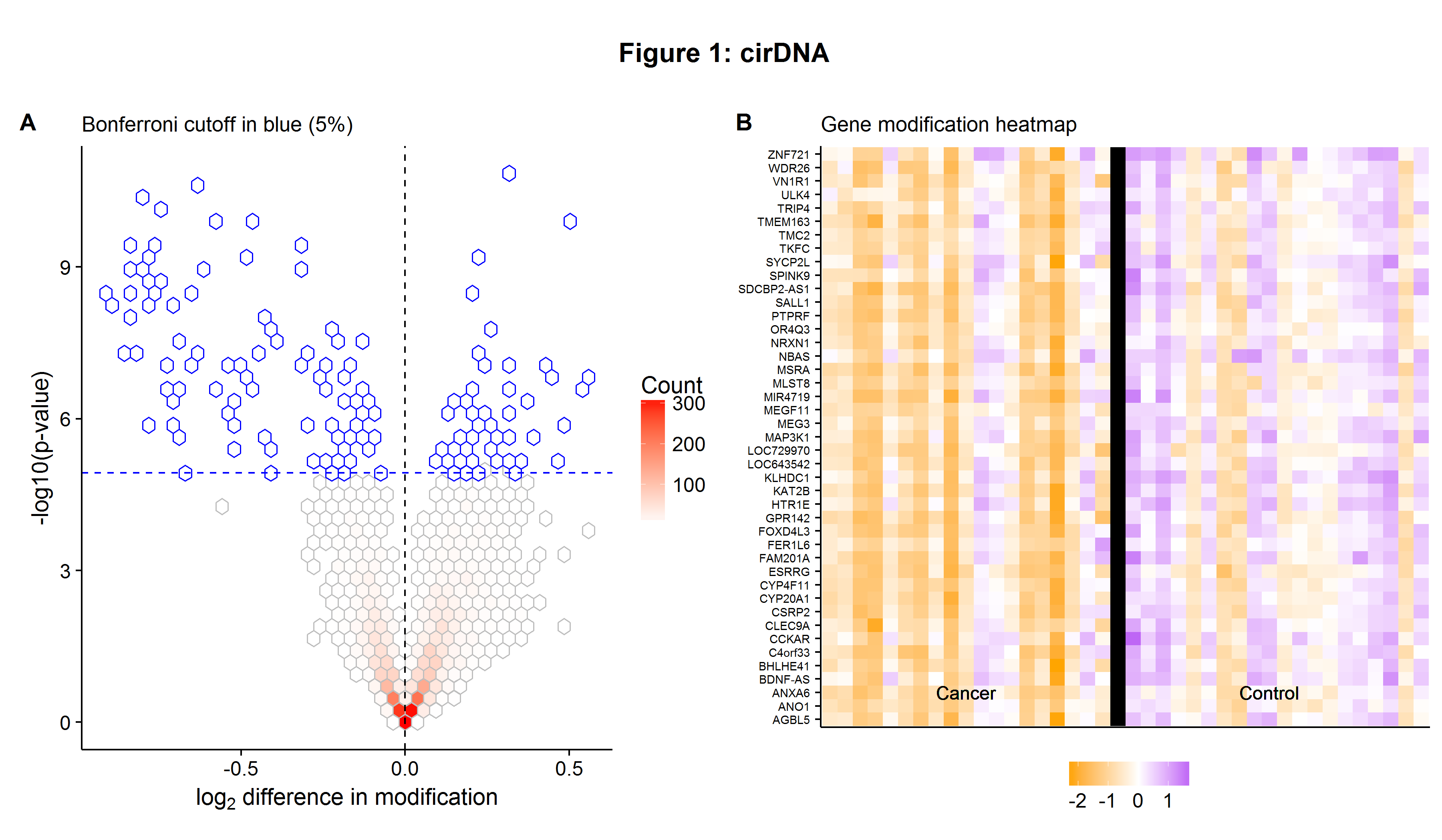
Figures 1A and 1B below are a Volcano plot and a heatmap similar to one seen in the original paper. The former shows the genes which are differentially modified as measured by a simple t-test between cancer and control samples. As multiple hypothesis tests are being conducted, the p-values need to be adjusted to take into account the false discovery rate[²]. The heatmap in Figure 1B shows some of the differentially modified genes that tend to be, relatively, under expressed in modification for cancer patients.

Desirable properties of a classifer

As Figure 1B shows, there are modification level differences between the two samples that would allow for the creation of a cancer/control classifier. However, the figure also shows that while these genes have a lower modification level for the cancer group, on average, there are some cancer (control) observations that are above (below) normal, showing that it is not a perfect signal. However, as this data set has \(N_{\text{Cancer}}=19\) and \(N_{\text{Control}}=20\), the data can be perfectly represented by 39 or more features; a simple exercise given there are \(p=4228\) gene loci. Building an accurate classifier therefore entails more than simply internally representing the 39 observations in a model form. Instead, a process that aims to measure predictive accuracy by emulating performance on a yet-to-be-seen test set is what is desired. Additionally, as all machine learning models contain hyperparameters that allow for a trade-off between bias and variance, this procedure must also be able to determine how the choice of these hyperparameter will generalize out-of-sample as well. In summary, the modelling pipeline needs to have two goals:

1. Determine the model which is most likely to have the best accuracy out-of-sample and what its associated optimal hyperparameters are.
2. Estimate what this accuracy rate is likely to be out-of-sample (this could include overall accuracy, as well as sensitivity and specificity).

A motivating example will elucidate the challenge. In all of these Monte Carlo simulations, the training set will be \(N=39\) for comparability to the cirDNA data set. Consider two data generating process (DGP) for binary outcomes: \(Y={ 0,1}\).

1. A totally random process: \(P(Y=1)=\pi\).
2. A simple logit process: \(P(Y=1 | X,\pmb{\beta})=\frac{1}{1+e^{-(\beta_0 + \beta_1 X)}}\), \(X \sim N(0,1)\).

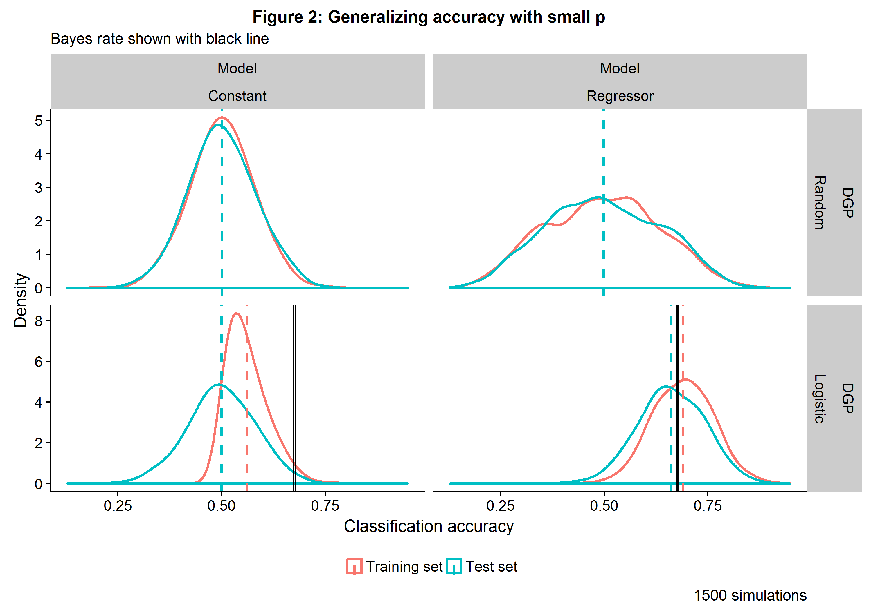
Two classifiers are considered: one that uses a constant (i.e. only information contained in the target variable) and one that uses a single covariate. The parameters of the logistic regression models are determined on a training set and then used to make predictions on both the training and the test set. Figure 2 below shows how well the two modeling approaches generalize their predictive accuracy on a training and test set of \(N=39\) each[³]. For the random DGP, the Constant model is equivalent to a coin toss and has an asymptotically normal distribution, whereas the Regressor model, while still unbiased, has a higher variance due to it using pure noise to make predictions.

When the DGP is itself generated with logistic distribution, the Constant model sees a better-than-random chance on the training data but reverts to a coin toss when predicting the test data (a result is to be expected as \(\beta_0=0\)). While the Regressor model has close to two-thirds accuracy, it nevertheless sees a slight dip in performance as it transitions from the training to the test set. The Bayes rate represents the best possible accuracy one could have had if the true probabilities were known. This simple Monte Carlo simulations reveals two important things:

1. Whenever a target variable is noisily observed, classification accuracy will be higher, on average, in the training set than on the test set.
2. No model can exceed the Bayes error rate on a test set, on average, but can do so in the training set due to over fitting.

Simulating out-of-sample accuracy with CV

The discrepancy between training and test set accuracy will become worse as \(p\) increases. To account for this known bias, a data set can be split into a training, validation, and test set. A range of models/hyperparameters can be fit on the training set, the best model can be determined on a validation set, and then out-of-sample accuracy can be estimated with a test set. However, this ideal approach requires a large \(N\). A more efficient approach is to combine the training and validation set into a single block, and then use \(k\)-fold cross-validation (CV) to perform model selection. In this procedure, the combined training-validation data is split up into \(k\) (roughly) equal pieces, a model is fit to \(k-1\) of the pieces, the predictive accuracy is recorded on the \(k^{th}\) left out piece, and the process is repeated for all \(k\) blocks. While this approach can provide an unbiased estimate of the best model and out-of-sample accuracy, it still requires enough data to be able to hold some aside for a test set. As the cirDNA data set has only \(N=39\), additional strategies beyond classical CV will be required for determining both model selection and the generalization of performance.

**The classical validation procedure with N is large**

In the following Monte Carlo simulations, there will be \(p=10\) features, \(N_{Train/Test}=39\) as before, and the logistic coefficient impacts for the DGP will be geometrically declining: \(\beta_k=(1/2)^k\), as in most data sets a few predictors account for a large share of the variation in the outcome. This set up nicely highlights the cost of model complexity: as the degrees of freedom decline linearly, information extracted increases at a decreasing rate (logarithmically), and there is some optimal point at which the additional information is not worth the cost.

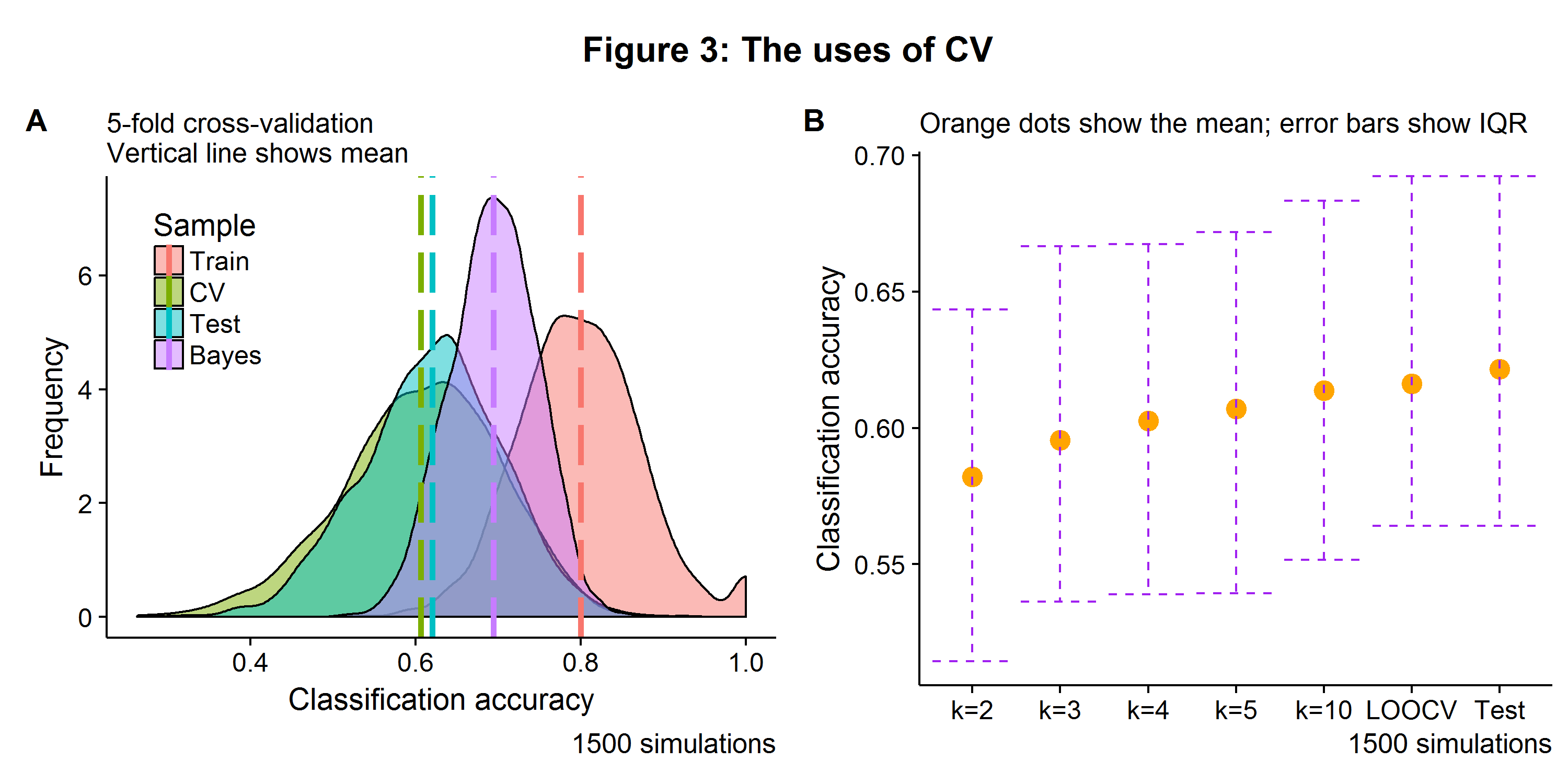
Figure 3A shows the distribution of the training, 5-fold CV, and test accuracy for a logistic regression model, as well as the Bayes error rate. Unsurprisingly the training error is well above the corresponding test error (due to over fitting). The CV error is a touch below the test error. Why is this? This is because the CV models were fit on \(\Big(\frac{k-1}{k}\Big)N\) observations, so the estimator had a fewer examples from which to learn from. However, this can be ameliorated by using Leave-one-out cross-validation (LOOCV), where \(k = N\), the approach which leads to the closest average approximation of the generalization error. However, in addition to a longer compute time, LOOCV will also have a higher variance for its validation predictions (there being no free lunch in statistics). Figure 3B shows that LOOCV is almost identical to the test error that would have been recorded on an unseen \(N_{\text{Test}}=39\) data set. In summary, using \(k\)-fold CV can provide an reasonable estimate of the test generalization error that would be seen on a new data set when testing a single model[⁴].

Performing model selection with CV

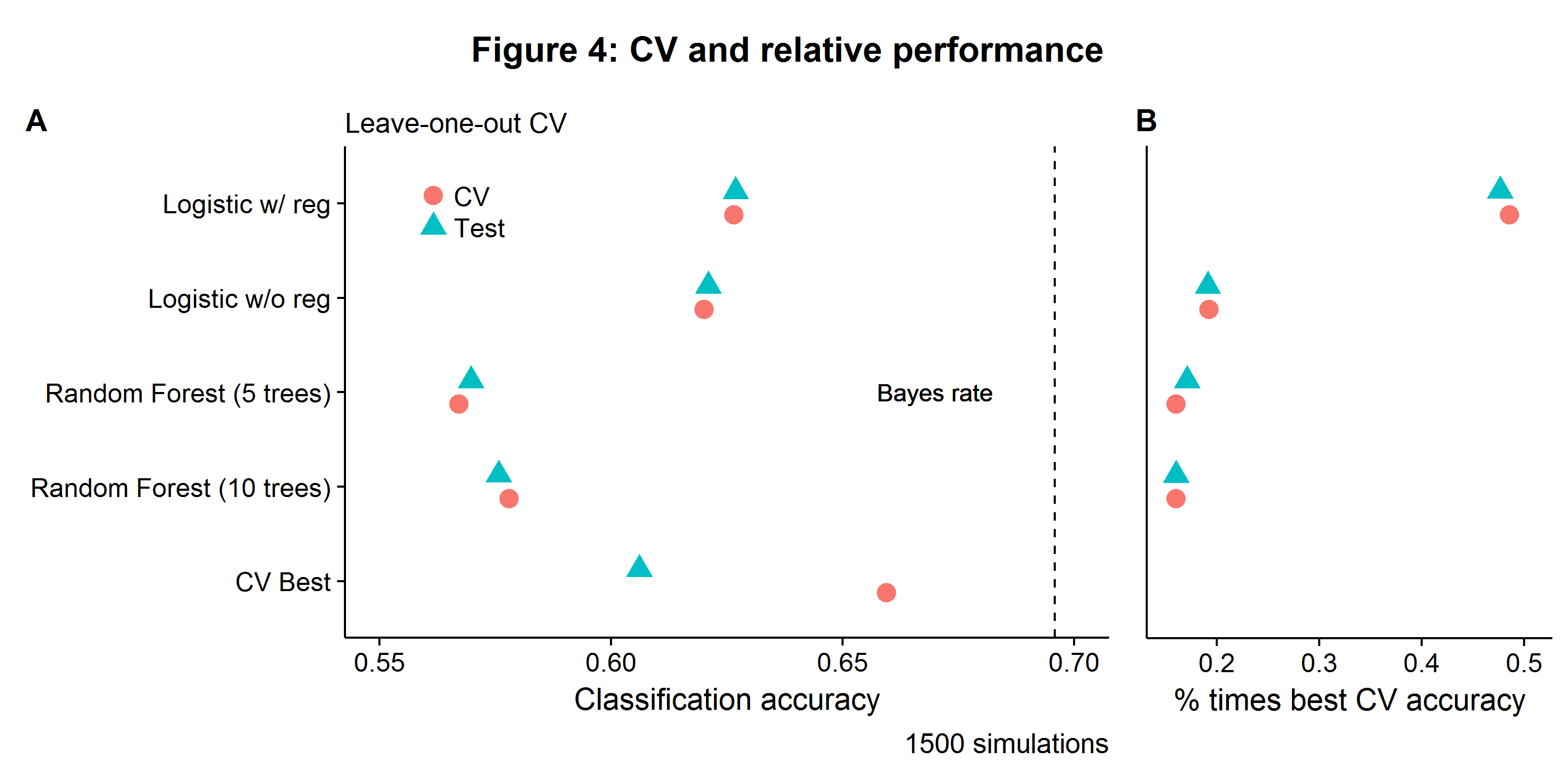
When only one model is used, LOOCV will answer the question of what the expected test set error will be. When there are several model hypotheses under consideration[⁵], the distribution of CV scores by model will provide an estimate of relative model performance out-of-sample, but will no longer provide an unbiased estimate of how the winning model will generalize on an unseen data set from the same DGP. Consider the trivial example of two random classifiers. Each model’s CV error will be 50% (on average) and the first random classifier will be beat the second’s CV score 50% of the time (on average). If the best performing model was chosen, then each model would be selected 50% of the time, which is an unbiased ratio of their relative performance. However, the average winning CV score will exceed 50% because the minimum of the two random models’ CV score is being selected, which is no longer random. Using the same DGP from the previous example, four models will be compared: two logistic regressions (one with and without some regularization) and two random forests (with five and ten trees, respectively).

Figure 4A shows the LOOCV error and associated test error, which are approximately equivalent for the four models. Relative model performance is reflected in how often each model is likely to be selected as having the highest CV accuracy, as seen in Figure 4B. The expected test set accuracy from performing model selection with the CV procedure is the weighted sum of model-specific accuracy and selection probability. For this DGP, the logistic model with some regularization has the best CV accuracy and test accuracy, on average, between the four models and gets selected about half of the time. However, the CV error associated with the best model for a given simulation is higher than its respective test error. Again, this is because once a model is selected the distribution of results is no longer random as there is data snooping going on.

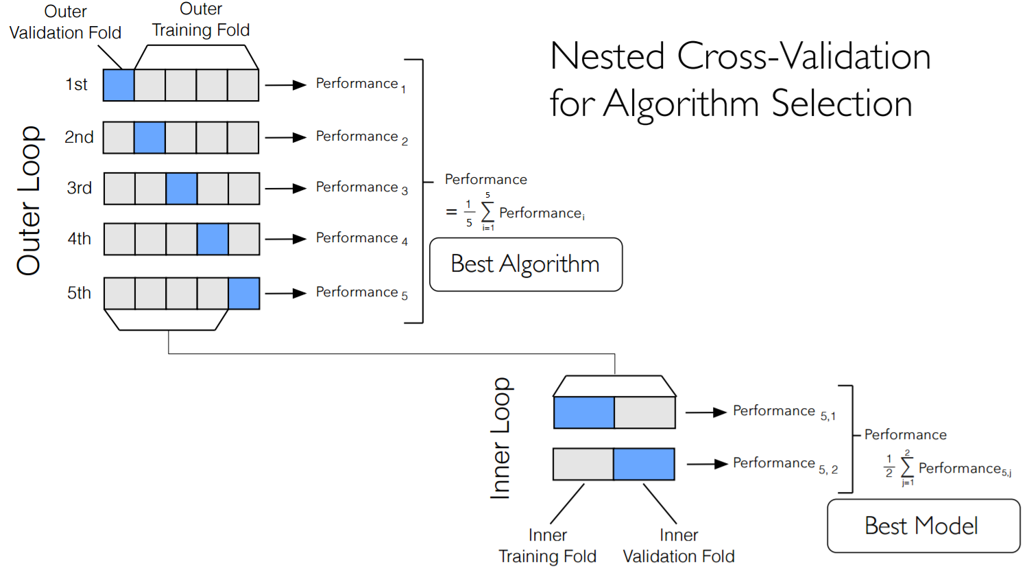
Is model selection via CV akin to Heisenberg’s uncertainty principle, whereby one can know the best model, or the approximate out-of-sample accuracy, but not both at the same time? It depends! For a large \(N\), the best model can be found by using the training-validation set, and a clean test set can be put aside whose only purpose is to determine how well a model’s accuracy will generalize to a new data set. When \(N\) is small, a technique known as nested CV can be used as a compromise between these two goals (see Crawley and Talbot (2010) for a further discussion of related issues). In the Cortese et al. (2012) paper, nested CV was used for fitting a random forest classifier to the data[⁶]. Nested CV works by running an inner and out validation loop: for a given iteration of the outer loop, one fold of data is put aside (the outer fold), and then rest of the data is then itself split up into multiple inner folds, where CV is used to evaluate the optimal parameters/model types under consideration (see diagram below). Even though the winning inner CV accuracy scores will be overly optimistic (for the reasons discussed previously), we can still learn about the accuracy of the overall machine learning process.

Specifically, if nested CV has \(k_1\) outer folds and \(k_2\) inner folds, then there will be \(k_1\) surrogate models (the parameterizations/model-types that won the inner CV competition on \(k_2\) folds). The accuracy of these \(k_1\) “winning models” on the held-out outer folds will closely approximate the true generalization error. Furthermore, the distribution of winning models will emulate the frequency at which these model types would be selected for (as seen in Figure 4B). Therefore nested CV represents an estimate of the generalization accuracy of a given machine learning pipeline. Therein lies the rub: nested CV can only provide an estimate of test set accuracy for the entire learning procedure, rather than for a given model at a single hyper-parameter value. Note that the final recommended model can simply be selected by performing CV on the whole data set. However, it would be incorrect to say that the resulting individual model will have the average of the outer CV accuracy.

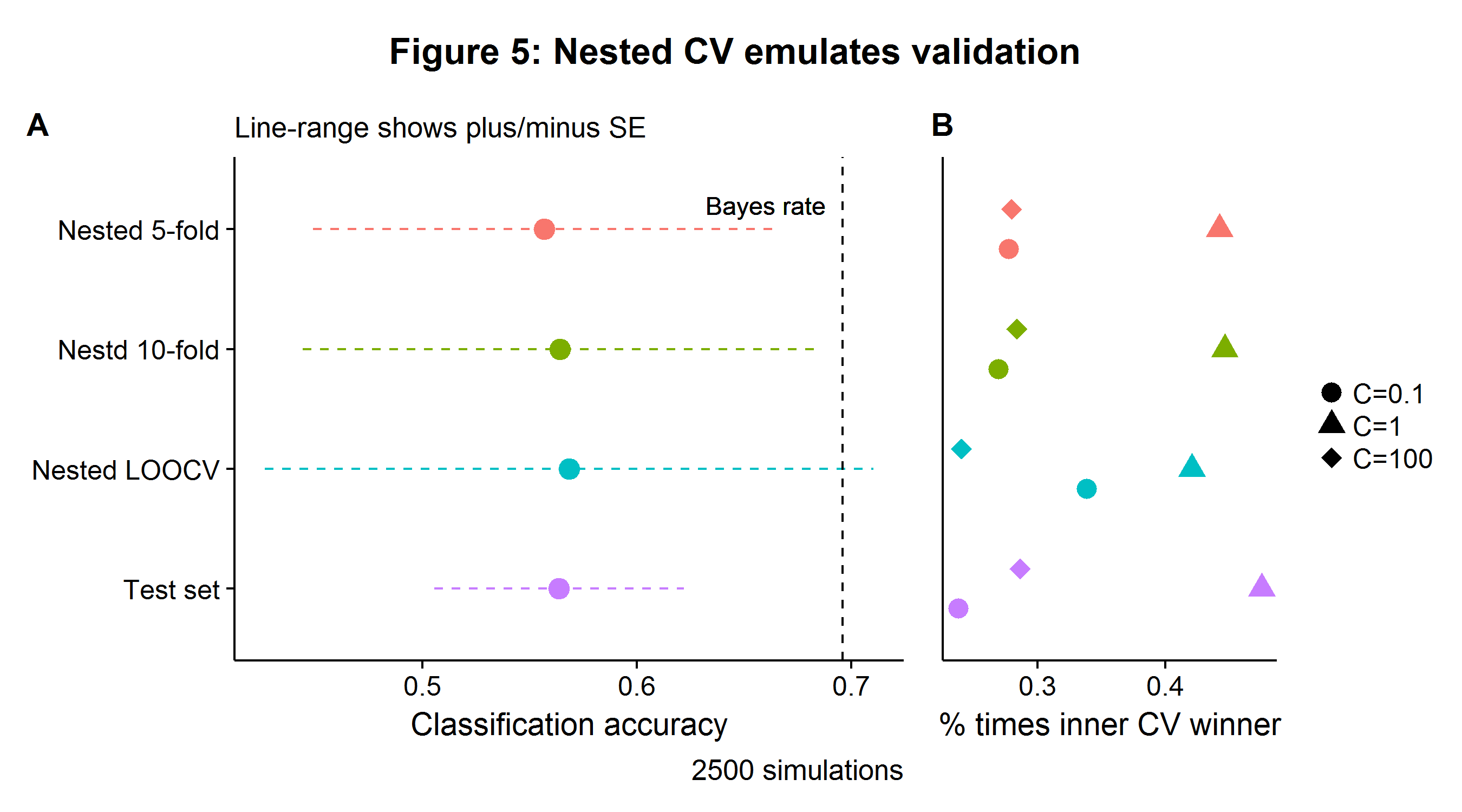
The next example will continue to use the previous DGP but with \(p=39\) features instead. Consider a machine learning pipeline which runs a nested CV procedure with five inner and outer loops for a logistic LASSO with three values of \(C={0.1,1,100}\), which are an inverse regularization parameter (increases in \(C\) lead to more model complexity)[⁷]. Equation \(\eqref{eq:lasso}\) shows the minimization problem for the logistic LASSO, where \(w\) is the vector of linear weights.

\[\begin{align} \min_{w,b} \|w\|_1 + C \sum_{i=1}^n \log(\exp(-y_i(X_i^T w + b))+1) \tag{1}\label{eq:lasso} \end{align}\]

The Monte Carlo simulations were carried out for two tracks: one using nested CV with \(N=39\) and one with \(N_{\text{Train}}=39\) and \(N_{\text{Test}}=39\) for a benchmark. Figure 5A and B shows that nested CV is able to closely match the results from a larger data set with a training and test split, albeit with more variance (there being no free lunch). In terms of the optimal number of folds, the nested LOOCV appears to have too much variance (in addition to a longer compute time), and I would opt for using 5- or 10-fold nested CV.

Note that if the researcher were to only consider the surrogate model scores of the model that won the plurality of inner loop competitions, then this would increase the average recorded score towards the best model’s unbiased generalization accuracy. However, this is not advisable as doing so comes at the price of even higher variance (as data is being thrown away), as well as other issues[⁸]. In summary, when the entire outer CV results are used, nested CV can provide an estimate for the average pipeline accuracy, as well as the relative performance of the different models under consideration. For this simulation, the logistic LASSO tuned with three regularization values of \(C\) achieves a classification accuracy of 56.7%, with the \(C=1\) parameter being selected the most often.

Building a cancer classifier with the cirDNA data set

When using nested CV, one wants to limit the number of model hypotheses under consideration for both interpretability and stability, especially when \(N=39\)[⁹]. The best model class for building a cancer classifier will depend on the nature of the DGP, including the relationship between features (covariance) and their correlation with the target (cancer). It is extremely important to not test any model or perform any feature selection outside of the model-evaluation stage. Doing so will lead to biased results (see Ambroise and McLachlan (2002))[¹⁰]. However, examining important statistics from the data can provide information about which machine learning model to choose. Figure 6A shows the (ordered) correlation coefficients between the \(p=4228\) gene loci and the outcome variable (cancer is coded as 1) when compared to a completely random data set of the same size. The B figure shows the difference in the correlation magnitude. Most of the signal appears to embedded in the first 275 features. However, these same features are also highly correlated, and a principal components (PC) decomposition reveals that the first two components account for most of the variation (Figure 6C).

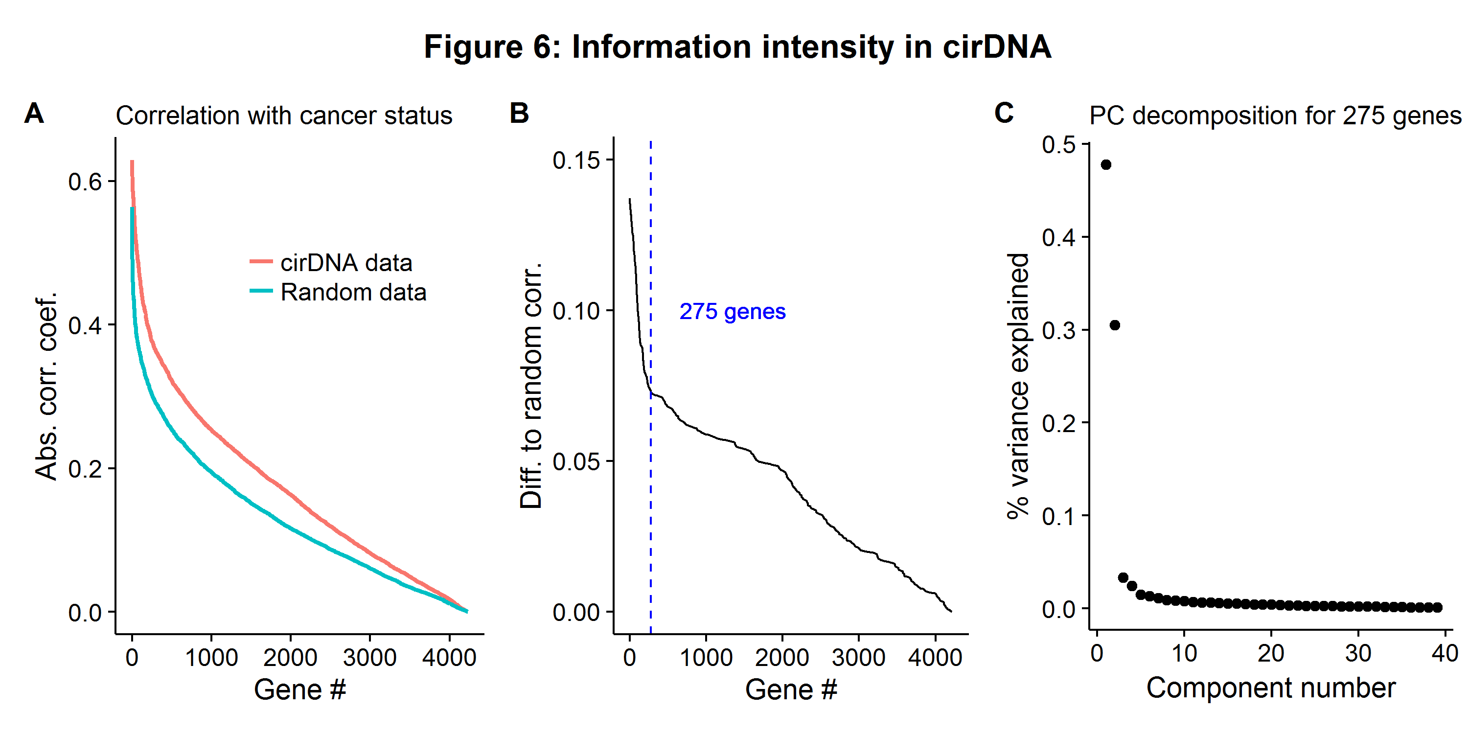
While having small amounts of information embedded in many variables suggests the use of a model with many features but highly shrunken coefficients like ridge regression or a boosted process, because the variables are also highly correlated, this suggests the use of a sparse learner. Therefore the logistic LASSO is opted for, as described in equation \(\eqref{eq:lasso}\). The learning pipeline will be as follows:

1. Remove any features that have missing values, zero variance, or are extremely unbalanced (i.e. have only a few unique values). This must be done as during the CV procedure, there can’t be a vector of zeros on one side of the split.
2. Calculate the normalizing weights for each gene, and then standardize the features.
3. Run a nested 5-fold outer and 10-fold inner CV on a logistic LASSO ranging from 1 to 10 degrees of freedom (i.e. the values of \(C\) on the LASSO solution path that lead from 1 to 10 variables with non-zero coefficients).
4. Report outer CV accuracy as the generalization error.
5. Use 5-fold CV to determine the final logistic LASSO model.

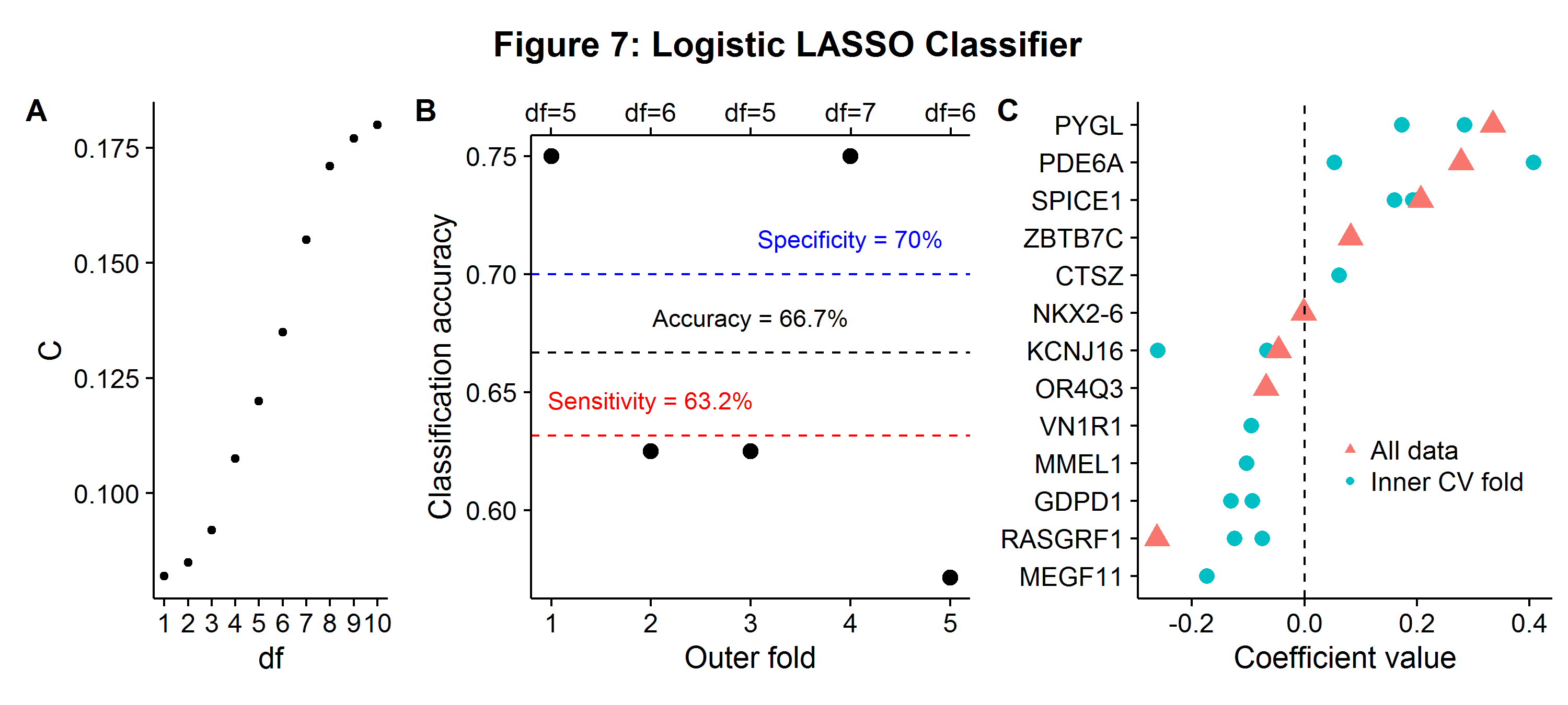
In stage 1 there end up being no features that need to be removed for technical reasons. Figure 7A shows the solution path of the logistic LASSO for the values of \(C\) associated with a given degree of freedom. The overall accuracy, sensitivity (true positive rate), and specificity (true negative rate) is shown in Figure 7B. The classifier correctly predicts two-thirds of the cases (66.7%), but is slightly better at distinguishing non-cancer (specificity: 70%) to cancer patients (sensitivity: 63.2%). The relative balance between sensitivity and specificity can be changed by assigning different weights to each outcome in the loss function. The same figure also shows the winning degrees of freedom from the inner CV competition, which range from 5 to 7 features. The close distribution of winning hyperparameters suggests a stable learning pipeline. Lastly, Figure 7C shows the non-zero coefficients for each gene loci that were used by the logistic LASSO in either the winning inner CV procedure or the final estimated model (df=8). This is another advantage of sparsity, the results are highly interpretable and can be used for further scientific research.

Overall, these results do not suggest that this classifier will have much production value as the accuracy rates are too low for a high stakes diagnosis. Furthermore, the accuracy rate is slightly lower than the one found in the original paper, suggesting that non-linear relationships between differentially expressed genes may be appropriate. However, this result is likely influenced by paucity of data. With additional cirDNA samples a more complex classifier could be trained to extract information from differentially modified genes between cancer and control samples.

---