When fitting a distribution to a survival model it is often useful to re-parameterize it so that it has a more tractable scale[¹]. However, estimating the parameters that index a distribution via likelihood methods is often easier in the original form, and therefore it is useful to be able to transform the maximum likelihood estimates (MLE) and its associated variance. However, a non-linear transformation of a parameter does not allow for the same non-linear transformation of the variance. Instead, an alternative strategy like the delta method must be employed. This post will detail its implementation and its relationship to parameter estimates that the survival package in R returns. We will use the NCCTG Lung Cancer dataset which contains more than 228 observations and seven baseline features. Below we load the data, necessary packages, and re-code some of the features.

library(survival); data(cancer)
lc <- tbl_df(cancer) %>% mutate(status2=ifelse(status==1,'Censored','Dead'),
                                    sex2=ifelse(sex==1,'Male','Female'),
                                censored=ifelse(status==1,1,0),
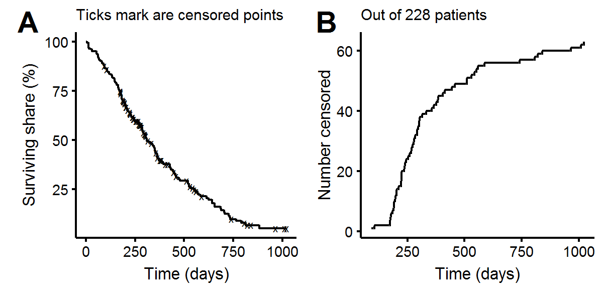
                                observed=ifelse(status==2,1,0))

To get a feel for the data set, we’ll create some KM curves. Plot A below shows the aggregate KM curve, with most patients having died within a three year period. Plot B shows that most of the censored observations occur between 1-2 years, which does not augur well for overall survival as most patients seem to live an extra year (of course there could be systematic feature differences between censored/uncensored patients which is why proper inference needs to be done with a multivariate procedure).

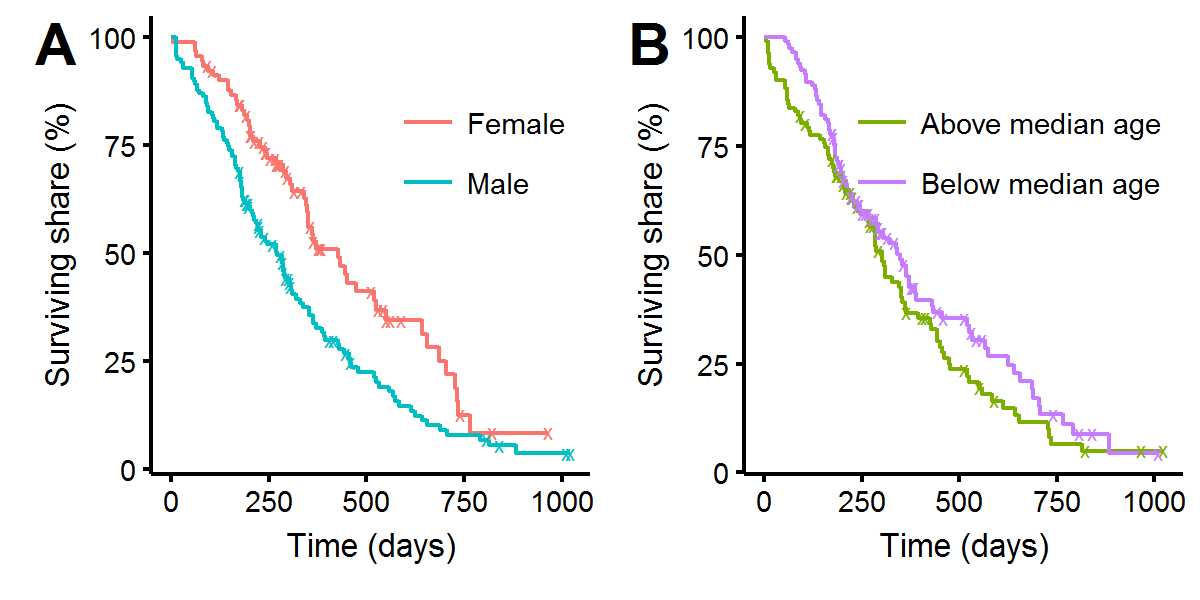
Plotting the KM curves for different categories of data can reveal associations between baseline features and relative survival rates. In figure A, we see that men have a higher mortality rate up until around day 750. There does not appear to be a significant difference between whether the patients were above or below the median age, as figure B shows, and this intuition is confirmed with a log-rank test: p-value=0.17.

Using the exponential distribution

As a warm-up, we’ll begin with the exponential distribution. While it is a somewhat unrealistic time-to-event distribution as it assumes a constant hazard rate (the conditional risk of transitioning from life to death stays the same over time), it is exceedingly tractable and good for demonstration purposes. The likelihood for any censored distribution is the joint distribution of the uncensored \(f(t|\theta)\) and censored \(P(T>t|\theta)=1-P(T<t|\theta)=1-F(t|\theta)\) observations. 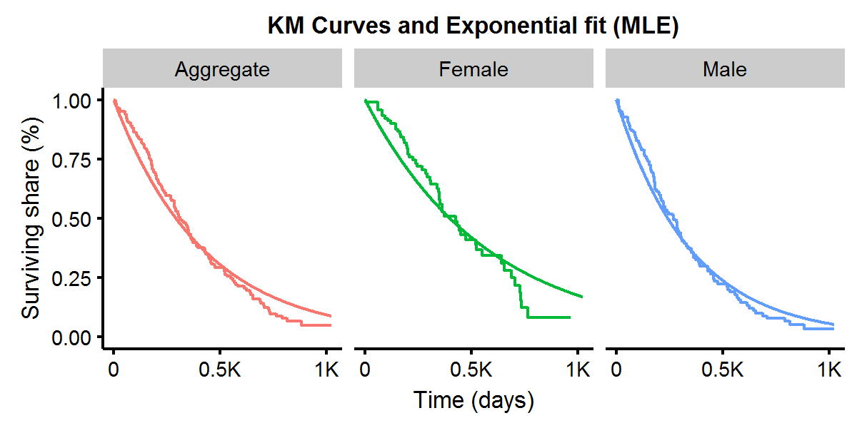Some additional notation: \(\lambda\) is the parameter indexing the exponential distribution, \(U(\lambda)\) is the score vector (it’s only a scalar in this case as the exponential distribution has only one parameter), \(I(\lambda)\) is the information matrix, and \(\delta_i\) is an indicator for whether or not the observation was censored.

Finding where the score (i.e. gradient) is equal to zero produces our MLE: \(\hat{\lambda}=\sum_i \delta_i/\sum_i t_i\). It is well known that the asymptotic variance of the MLE is the corresponding point in the inverse information matrix: \(Var(\hat{\lambda})=I^{-1}(\hat{\lambda})\) and so \(SE(\hat{\lambda})=\sqrt{\sum_i \delta_i}/\sum_i t_i\), which is a fairly tidy expression! We can see that our estimate of \(\lambda\) is therefore: 9.1e-04 with a SE of 1.1e-04 (very small numbers). Let’s plot what this exponential distribution looks like compared to the aggregate KM curve. As we can see below the parametric survival curve with the MLE estimate of \(\lambda\) does a fairly decent job approximating the non-parametric KM curve.

However, to make the scale of \(\lambda\) more tractable, we could do a log transformation: \(\alpha=-\log(\lambda)\), which implies that \(\lambda=\exp(-\alpha)\). Next, to perform inference on \(\alpha\) using the information from the likelihood for \(\lambda\), we appeal to both:

1. The invariance property of the maximum likelihood estimator: \(\hat{\alpha}_{\text{MLE}} = g(\hat{\lambda}_{\text{MLE}})\)
2. The Delta method: \(\begin{aligned} Var(g(\lambda)) &= [g'(\lambda)]^2 Var(\lambda) \\ SE(g(\lambda)) &= | g'(\lambda)] | SE(\lambda) \\ \end{aligned}\)

The invariance property says that if there exists a function \(g(\lambda)\) which is one-to-one, then the MLE of this function of \(\lambda\) is simply the function evaluated at the MLE of \(\lambda\). The delta method provides a way to relate the variance of a function of a random variable (or estimator) to that variable/estimator when it is asymptotically normal. In our case \(g’(\lambda)=-1/\lambda\) and hence:

Implementing this in R:

# Calculate the MLE point estimate and se
mle.lam <- sum(lc$observed)/sum(lc$time)
se.lam <- sqrt(sum(lc$observed))/sum(lc$time)
# Print the delta method results
data.frame(alpha=-log(mle.lam),se=(1/mle.lam)*se.lam)

##      alpha         se
## 1 6.044474 0.07784989

Finally, we can see the relation of the delta method to the survival package. When we use the survreg function we see that the exponential distribution is parameterized as the \(\alpha\) we discussed above.

# Create Surv object
lc.Surv <- Surv(time=lc$time,event=lc$status2=='Dead',type='right')
# Estimate with R
summary(survreg(lc.Surv~1,dist='exp'))$table

##                Value Std. Error        z p
## (Intercept) 6.044474 0.07784989 77.64267 0

A bivariate distribution: the Weibull

As a more advanced example, consider the following parameterization of the Weibull distribution with \(\theta=(p,\lambda)\) for the following density and survival functions:

Solving for the log-likelihood:

Which we see reduces to the log-likelihood of the exponential distribution when \(p=1\), and hence the exponential is embedded in the Weibull. Finding the Score vector:

And the information matrix:

We’ll ask R to find the pair of \((\hat{p},\hat{\lambda})\) that minimizes the (negative) of our log-likelihood using the optim function.

# Get data vectors
tt <- lc$time
delta <- lc$observed
# Function to minimize
ll <- function(x,delta,tt) { 
  x1 <- x[1] # p
  x2 <- x[2] # lam
  -1*( sum( delta*(log(x1) + log(x2) + (x1-1)*log(tt) ) - x2*tt^x1 ) )
}
# Gradient
U <- function(x,delta,tt) {
  x1 <- x[1] # p
  x2 <- x[2] # lam
  -1*c( sum(delta)/x1 + sum(delta*log(tt)) - x2*sum(tt^x1 * log(tt)),
        sum(delta)/x2 - sum(tt^x1) )
}
# MLE estimates of p/lambda
plam.mle <- optim(par=c(2,0.001),fn=ll,gr=U,tt=tt,delta=delta,
      control=list(reltol=1e-20))
p.mle <- plam.mle$par[1]
lam.mle <- plam.mle$par[2]

The inverse of the information matrix evaluated at the MLE point estimates provides an estimate of the standard errors.

# Define the information matrix
I.weibull <- function(p,lam,delta,tt) {
  matrix(c( sum(delta)/p^2 + lam*sum(tt^p * log(tt)^2 ), sum(tt^p * log(tt)), 
               sum(tt^p * log(tt)), sum(delta)/lam^2 ),ncol=2)
}
# Get standard errors
plam.se <- I.weibull(p=p.mle,lam=lam.mle,delta,tt) %>% solve %>% diag %>% sqrt
p.se <- plam.se[1]
lam.se <- plam.se[2]
# Print
data.frame(p=c(p.mle,p.se),lambda=c(lam.mle,lam.se)) %>% 
  set_rownames(c('Estimate','S.E.')) %>% round(5)

##                p  lambda
## Estimate 1.31684 0.00035
## S.E.     0.08221 0.00018

Below we can see that these estimates minimize the log-likelihood.

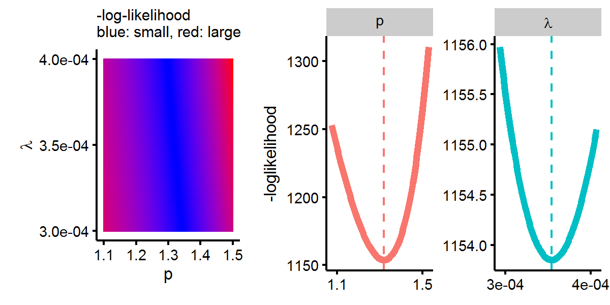
Next we’ll estimate the same Weibull model but using the survreg function. The survival package parameterizes the Weibull distribution so that the survival function takes the following form: \(S(t)=\exp{ -(e^{-\alpha} t)^{1/\beta} }\). Hence we can see that the relation to our parameterization is \(p=1/\beta\) and \(\lambda=\exp{-\alpha/\beta }\). Let’s estimate the model and make sure the results map back to each other.

# Estimate Weibull parameters with survreg
weibull.survreg <- survreg(lc.Surv~1,dist='weibull')
weibull.survival <- summary(weibull.survreg)$table
a.w <- weibull.survival[1,1]
blog.w <- weibull.survival[2,1]
b.w <- exp(blog.w)
# Convert back
p.w <- 1/b.w
lam.w <- exp(-a.w/b.w)
# Compare
data.frame(mle=c(p.mle,lam.mle),survreg_transform=c(p.w,lam.w)) %>%
  set_rownames(c('p','lambda')) %>% round(5)

##            mle survreg_transform
## p      1.31684           1.31684
## lambda 0.00035           0.00035

Great so the results are comparable. However suppose we want to convert the standard errors the survreg object returns to \(p\) and \(\lambda\)? First notice that the survreg object returns the estimate of the variance-covariance matrix for \([\alpha,\log\beta]\).

var.alogb <- weibull.survreg$var
var.alogb

##               (Intercept)    Log(scale)
## (Intercept)  3.497056e-03 -8.903365e-05
## Log(scale)  -8.903365e-05  3.897543e-03

We can use the multivariate delta method to transform this back to \(Var(\alpha,\beta)\).

In the first case case \(g(\alpha,\beta)=[g_1(\alpha,\beta),g_2(\alpha,\beta)]=[\alpha,\log\beta]\), and \(J(\alpha,\beta)\) is the Jacobian matrix, which will be:

# Define the jocabian for g(alpha,beta) = (alpha, log(beta))
J.alogb <- matrix(c(1,0,0,1/b.w),ncol=2)
# Get the variance of a,beta
var.ab <- solve(J.alogb) %*% var.alogb %*% solve(J.alogb)

Next we use the same multivariate delta method except now for \(h(\alpha,\beta)=[1/\beta,\exp{-\alpha/\beta}]=[p,\lambda]\), and hence the Jacobian will be:

Solving in R:

# Get the Jacobian for p/lambda
J.plam <- matrix( c(0, -1/b.w*exp(-a.w/b.w), -1/b.w^2, a.w/b.w^2*exp(-a.w/b.w)) ,ncol=2)
# Get the variance of p/lambda
var.plam <- J.plam %*% var.ab %*% t(J.plam)

Now we’ll confirm that the square-roots of the diagonals line up with our previous estimate of the standard errors derived from the inverse of the information matrix:

# Compare to our SE based on information matrix approach
data.frame(se.delta=var.plam %>% diag %>% sqrt,
           se.mle=c(p.se,lam.se)) %>%
  set_rownames(c('p','lambda')) %>% round(5)

##        se.delta  se.mle
## p       0.08221 0.08221
## lambda  0.00018 0.00018

Great! We have successfully shown how the delta method can be used to derive the standard errors for any re-parameterization. We have also seen how the SEs derived from the delta method relate to the maximum likelihood estimator and the output that certain R packages return.