
Using a modified Hausman likelihood to adjust for binary label error
(1) Overview
In most statistical models randomness is assumed to come from a parametric relationship. For example, a random variable \(y\) might have a Gaussian \(y \sim N(\mu,\sigma^2)\) or exponential distribution \(y \sim \text{Exp}(\lambda)\) centred around some point of central tendency \(E[y] = \mu\) or \(E[y] = \lambda^{-1}\). Conceptually, we tend to think of the observed value of a random variable comprising of two parts: a fixed component and an idiosyncratic random element: \(E[y] = f(\mu) + e\). Human height can be thought of as a function genetics (fixed) and all other environmental influences (idiosyncratic). However, when the data is actually collected and recorded, a further element of randomness can also be introduced: measurement error. For example, in a database of human height, each observation will be equal to the individual’s actual height, plus some error due to the measuring process. For real datasets, it is likely that a large share, if not the majority, contain both kinds of randomness.[1]
In most applied statistical settings, the problem of measurement error is either ignored or misunderstood. The consequence of disregarding this issue will depend on the nature of the quantity being estimated. In the presence of classical measurement error for a linear regression model, measurement error on the response leads to increased variance while measurement error on the covariates leads to shrunken coefficients. The latter phenomenon is not unrelated to a principle machine learning researchers have known for a long time: adding noise to input features is equivalent to regularization (and can explicitly be shown to mimic Ridge regression). When the outcome variable is binary, the consequence of measurement error on either the response or the covariates is regularized coefficients. Unfortunately, the knowledge that measurement error usually leads to shrunken coefficients has given applied statisticians undue confidence in their estimates. As Jerry Hausman expressed:
I have called this the “Iron Law of Econometrics” - the magnitude of the estimate is usually smaller than expected. It is also called “attenuation” in the statistics literature.
This sentiment has encouraged the “What does not kill my statistical significance makes it stronger” fallacy. Even though covariate mismeasurement may lead to conservative estimates, it does not solve the more general problem of statistical significance filters and a winner’s curse phenomenon for published effect sizes. Furthermore, when the measurement error is correlated with the response or with other observations the standard consequences of attenuated coefficients no longer holds.
However, when it is possible to correct for measurement error, a statistician should always do so. If some of the features have been imputed due to missing data, using errors-in-variables techniques can help to obtain more precise inference. Recently, econometric studies have been using machine learning models to impute binary features or outcomes based on some pre-trained models. Because they often fail to adjust for the known classification error rates, these studies leave unused statistical information on the table. In biostatistics literature, a recent paper has referred to this problem as doing post-prediction inference.
To help researchers adjust for measurement error in binary labels this post will provide the python code needed to implement a likelihood formulation as proposed in Hausman’s 1998 paper. While the code will primarily be useful for the problem of doing traditional statistical inference, it can also be easily adapted to deep learning models (I provide equivalent functions using automatic differentiation in section 6) and other applications such as label feedback loop problems. The code in this post is selectively shared, and if you are interested in replicating all figures and results, please see this repo.
(2) The consequence of classical measurement error
It is worth reviewing the effects of classical measurement error for both logistic and linear regression models:
\[\begin{align*} P(y_i = 1) &= \sigma(\eta_i), \hspace{5mm} \text{Logistic} \\ \sigma(z)&=1/(1+\exp(-z)) \\ y_i &= \eta_i + e_i, \hspace{5mm} \text{Linear} \\ e_i &\sim N(0,\tau^2) \\ \eta_i &= x_i^T \beta \end{align*}\](2.A) Covariate measurement error
When features are mismeasured with zero-centred Gaussian noise, we refer to this as classical measurement error on the covariates. Specifically: \(x_{ij}^{\text{obs}} = x_{ij} + u_{ij}\), \(u_{ij} \sim N(0, \gamma^2)\). The presence of this measurement error leads to attenuated coefficients and standard errors as well as conservative z-scores for both logistic and linear regression.[2]
Figure 1: Effect of measurement error on the covariates
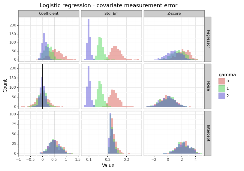
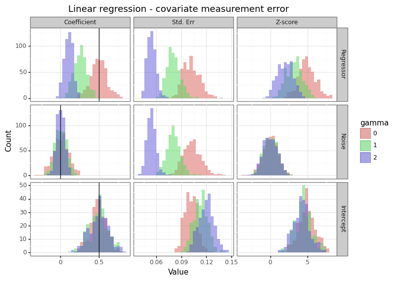
This is the most benign type of measurement error because it effectively acts as regularization (similar to the way a prior does in Bayesian inference). When a column is stochastically unrelated to the response, adding noise (\(\gamma\)) will reduce the magnitude of statistically significant findings. The winner’s curse problem is diminished with this type of noise.[3]
(2.B) Label measurement error
Next, we will see how measurement error for the response variable impacts statistical inference.
\[\begin{align*} P(y_i^{\text{obs}} = 1) &= \sigma(\eta_i + u_i), \hspace{5mm} \text{Logistic} \tag{1}\label{eq:noise1} \\ y_i^{\text{obs}} &= y_i + u_i = \eta_i + e_i + u_i, \hspace{5mm} \text{Linear} \\ u_i &\sim N(0, \gamma^2) \\ \end{align*}\]To allow for consistent comparisons between the logistic and linear models, the label noise in this formulation occurs through skewing the logits (and hence probabilities) of the underlying logistic distribution \eqref{eq:noise1}.
Figure 2: Effect of measurement error on the response
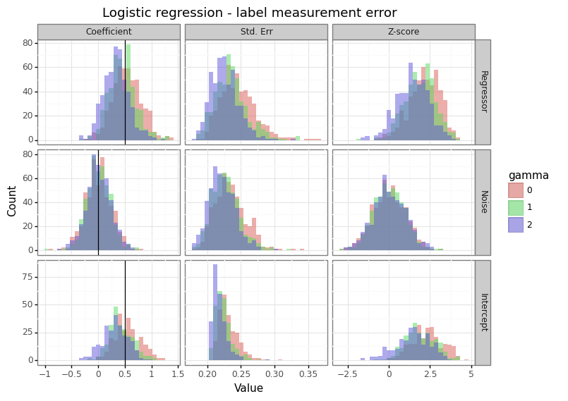
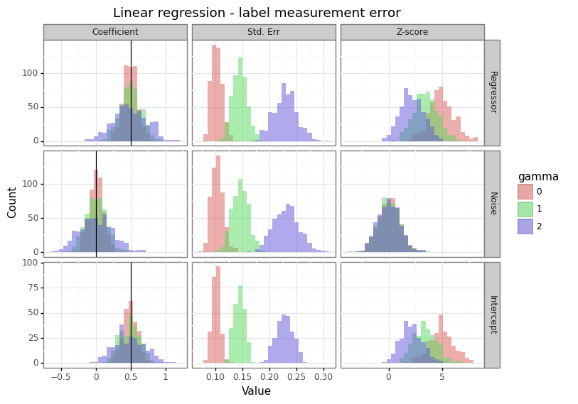
Unlike the case of covariate measurement error, the consequence of label measurement error for logistic and linear regression differs. For logistic regression, features with non-zero coefficients attenuate towards zero, whilst covariates with no relationship to the response maintain their (zero-centred) distribution. For linear regression however, the increase in label variance causes the variation in coefficient estimates to expand. This means that measurement error in the response exacerbates the winner’s curse phenomenon for statistically significant results.
In summary, even when the measurement error comes from a zero-centred Gaussian distribution, its effects will depend on whether it applies to the covariates or the label, as well as whether the underlying data generating process is linear or logistic. We can summarize these results as follows:
| Feature (model) | Covariate error | Label error |
|---|---|---|
| Regressor (logistic) | Regularization | Regularization |
| Noise columns (logistic) | Regularization | No effect |
| Regressor (linear) | Regularization | Increased variance |
| Noise columns (linear) | Regularization | Increased variance |
(3) Hausman estimator
Recall that in the previous formulation for logistic regression, the noise occurs within the inverse link function for the logistic model \eqref{eq:noise1}. One could also imagine the label error for a binary outcomes model occurring after the realization (i.e. “label flipping”), rather than through skewing the probabilities:
\[\begin{align*} y_i^{\text{obs}} &= \begin{cases} 1 & \text{ if } y_i = 1 \text{ with prob } 1-\alpha_1 \\ 0 & \text{ if } y_i = 1 \text{ with prob } \alpha_1 \\ 0 & \text{ if } y_i = 0 \text{ with prob } 1-\alpha_0 \\ 1 & \text{ if } y_i = 0 \text{ with prob } \alpha_0 \\ \end{cases} \tag{2}\label{eq:noise2} \end{align*}\]While there exists an equivalence between \eqref{eq:noise1} and \eqref{eq:noise2} for some choice of noise distribution \(u_i\sim N(\mu,\gamma^2)\), the label flipping framework of \eqref{eq:noise2} is more conceptually appealing and forms the basis of the modified likelihood method proposed by Hausman (1998).
\[\begin{align*} \alpha_0 &= P(y_i^{obs} = 1 | y_i=0 ) \hspace{1cm} \text{(FPR)} \\ \alpha_1 &= P(y_i^{obs} = 0 | y_i=1 ) \hspace{1cm} \text{(FNR)} \\ E[y_i | x_i] &= P(y_i=1 | x_i) = \underbrace{\alpha_0}_{\text{(FPR)}} + \underbrace{(1-\alpha_0-\alpha_1)}_{\text{(TPR)}} F(\eta_i) \tag{3}\label{eq:hausman} \end{align*}\]As equation \eqref{eq:hausman} shows, when the false positive rate (FPR) is above zero, this causes the expected value of observed binary labels to increase since some true zero labels are flipped to ones. In the same vein, an increase in the false negative rate (FNR) causes the observed label balance to decrease since some true ones are observed as zeros. Assuming one knew the true values of \(\alpha_0\) and \(\alpha_1\), one could obtain increasingly precise estimates of the coefficient parameters \(\beta\) by using this probabilistic formulation in the likelihood. When the data generating process (DGP) is a parametrized version of a Bernoulli distribution, the usual cross-entropy loss can carry out maximum likelihood estimation.
\[\begin{align*} a_{01} &= 1-a_0-a_1 \\ \bar{y}_i(\eta_i,a_0,a_1) &= E[y_i | x_i] = a_0 + a_{01}F(\eta_i) \\ \ell(\eta) &= \sum_{i=1}^n \big[ y_i \log(\bar{y}_i) + [1-y_i]\log(1-\bar{y}_i) \big] \\ \end{align*}\]To calculate the gradients of the log-likelihood function, I found it easiest to use the chain rule by taking the gradients with respect to the linear predictors first, and then the linear predictors with respect to \(\beta\).
\[\begin{align*} \frac{\partial \ell}{\partial \eta_i} &= a_{01} \cdot F'(\eta_i) \cdot \Bigg[\frac{y_i}{\bar{y}_i} - \frac{1-y_i}{1-\bar{y}_i} \Bigg] \\ \frac{\partial \ell}{\partial \eta} &= \begin{pmatrix} \frac{\partial \ell}{\partial \eta_1} & \frac{\partial \ell}{\partial \eta_2} & \dots & \frac{\partial \ell}{\partial \eta_n} \end{pmatrix}^T \\ \frac{\partial \ell}{\partial \beta} &= X^T \frac{\partial \ell}{\partial \eta} \\ \frac{\partial \ell}{\partial a_0} &= \sum_i (1-F(\eta_i))\cdot \Bigg[\frac{y_i}{\bar{y}_i} - \frac{1-y_i}{1-\bar{y}_i} \Bigg] \\ \frac{\partial \ell}{\partial a_1} &= \sum_i F(\eta_i)\cdot \Bigg[\frac{1-y_i}{1-\bar{y}_i} - \frac{y_i}{\bar{y}_i} \Bigg] \\ \frac{\partial \ell}{\partial \gamma} &= \begin{pmatrix} \partial \ell/\partial a_0 \\ \partial \ell / \partial a_1 \\ \partial \ell / \partial \beta \end{pmatrix}_{(p+2) \times 1} \\ \gamma &= \begin{pmatrix} a_0 & a_1 & \beta \end{pmatrix}^T \end{align*}\]The gradient matches the usual cross-entropy loss, the only difference being that \(\bar{y}_i\) is a function of \(a_0\) and \(a_1\) in addition to some sigmoid-like function \(F\). If \(F\) is the sigmoid function then \(F’=F(1-F)\), for example. The terms for the Hessian can be derived with a bit of extra work:
\[\begin{align*} \frac{\partial \ell^2}{\partial \eta_i^2} &= a_{01} \Bigg\{ F''(\eta_i)\Bigg[ \frac{1-y_i}{1-\bar{y}_i} - \frac{y_i}{\bar{y}_i} \Bigg] - a_{01} [F'(\eta_i)]^2 \Bigg[ \frac{y_i}{\bar{y}_i^2} + \frac{1-y_i}{(1-\bar{y}_i)^2} \Bigg] \Bigg\} \\ \frac{\partial \ell^2}{\partial \eta \partial \eta^T} &= \text{diag}\begin{pmatrix} \frac{\partial \ell^2}{\partial \eta_1^2} & \dots & \frac{\partial \ell^2}{\partial \eta_n^2} \end{pmatrix} \\ \frac{\partial \ell^2}{\partial \beta \partial \beta^T} &= X^T \Bigg[ \frac{\partial \ell^2}{\partial \eta \partial \eta^T} \Bigg]_{n \times n} X \\ \frac{\partial \ell^2}{\partial \eta_i \partial a_0} &= -F'(\eta_i) \Bigg\{ \frac{y_i}{\bar{y}_i} - \frac{1-y_i}{1-\bar{y}_i} + a_{01}(1-F(\eta_i))\Bigg[ \frac{y_i}{\bar{y}_i^2} + \frac{1-y_i}{(1-\bar{y}_i)^2} \Bigg] \Bigg\} \\ \frac{\partial \ell^2}{\partial \eta_i \partial a_1} &= F'(\eta_i) \Bigg\{ \frac{1-y_i}{1-\bar{y}_i} - \frac{y_i}{\bar{y}_i} + a_{01} F(\eta_i) \Bigg[ \frac{y_i}{\bar{y}_i^2} + \frac{1-y_i}{(1-\bar{y}_i)^2} \Bigg] \Bigg\} \\ \frac{\partial \ell^2}{\partial \eta \partial a_j} &= \begin{bmatrix} \frac{\partial \ell^2}{\partial \eta_1 \partial a_j} & \dots & \frac{\partial \ell^2}{\partial \eta_n \partial a_j} \end{bmatrix}^T_{n \times 1} \\ \frac{\partial \ell^2}{\partial a_j \partial \beta} &= X^T \frac{\partial \ell^2}{\partial \eta \partial a_j} \\ \frac{\partial \ell^2}{\partial a_0^2} &= - [1-F(\eta_i)]^2 \Bigg[ \frac{y_i}{\bar{y}_i^2} + \frac{1-y_i}{(1-\bar{y}_i)^2} \Bigg] \\ \frac{\partial \ell^2}{\partial a_1^2} &= - [F(\eta_i)]^2 \Bigg[ \frac{y_i}{\bar{y}_i^2} + \frac{1-y_i}{(1-\bar{y}_i)^2} \Bigg] \\ \frac{\partial \ell^2}{\partial a_0 \partial a_1} &= F(\eta_i)[1-F(\eta_i)] \Bigg[ \frac{y_i}{\bar{y}_i^2} + \frac{1-y_i}{(1-\bar{y}_i)^2} \Bigg] \\ \frac{\partial \ell^2}{\partial \gamma \partial \gamma^T} &= \begin{pmatrix} \frac{\partial \ell^2}{\partial a_0^2} & \frac{\partial \ell^2}{\partial a_0 \partial a_1} & \frac{\partial \ell^2}{\partial a_0 \partial \beta}^T \\ \frac{\partial \ell^2}{\partial a_1 \partial a_0} & \frac{\partial \ell^2}{\partial a_1^2} & \frac{\partial \ell^2}{\partial a_1 \partial \beta}^T \\ \frac{\partial \ell^2}{\partial a_0 \partial \beta} & \frac{\partial \ell^2}{\partial a_1 \partial \beta} & \frac{\partial \ell^2}{\partial \beta \partial \beta^T} \end{pmatrix} \end{align*}\]While I have used the sigmoid function \(\sigma\) for \(F\), other functions can be chosen such as the probit function. With these likelihood, gradient, and Hessian functions, any standard optimization routine can be used to find the parameters which minimize the (negative) log-likelihood. The original Hausman paper showed that parameters \((\alpha_0, \alpha_1, \beta)\) are identifiable and can be consistently estimated if \(F\) is non-linear and \(\alpha_0 + \alpha_1 < 1\). When \((\alpha_0, \alpha_1)\) are known or estimated in advance, these parameters can be fixed.
(4) Hausman model class
The code block below provides the necessary functions needed to carry out optimization of the Hausman-modified cross-entropy loss. I have structured the LogisticHausman class to match sklearn with fit, predict_proba, and predict methods. In addition, the inverse of the Hessian is used to calculate the standard errors (.se). When the model class is initialized, the user can specify whether \((\alpha_0,\alpha_1)\) should be fixed in advance, and if so, at what values (the default is zero). Hence, to obtain a normal logistic regression estimator, the class can be called as follows: mdl=LogisticHausman(fixed=True,a0=0,a1=0). There are several other attributes that can be set: i) add_int is a boolean as to whether a column of ones should be added to the x matrix, ii) F is some sigmoid-like function (default is the sigmoid function), and iii) thresh is the operating threshold to convert predicted probabilities into a one or a zero.
For those interested in the details of the optimization routine there are several notes to make. First, the loss, gradient, and Hessian functions are always based on the negative log-likelihood as we are using scipy’s minimize function. Second, the choice of CDF function (\(F(\cdot)\)) must allow for up to two orders of differentiation, since this is required for the calculation of the Hessian (as can be seen in the equations above). Third, when \((\alpha_0,\alpha_1)\) are being estimated, optimization bounds are placed to ensure they stay between zero and one. Fourth, I found that for small sample sizes the likelihood function can be very flat and it will result in convergence to large parameter values with a non-invertible Hessian. There is an L2-norm check on the coefficients, but more sophisticated methods such as early stopping or regularization could be used to help with identifiability in these situations.
import numpy as np
import pandas as pd
from funs_support import cvec
from scipy.optimize import minimize
from scipy.optimize import Bounds

def sigmoid(eta, order=0):
    if not isinstance(eta, np.ndarray):
        eta = np.array(eta)
    assert order >= 0 and order <= 2
    p = 1 / (1 + np.exp(-eta))
    if order == 0:
        return p
    elif order == 1:
        return p * (1-p)
    else:
        return 2*p**3 - 3*p**2 + p


# ------- FIXED A0/A1 ------ #

def nll_hausman_fixed(bhat, y, X, F, a0, a1):
    a01 = (1-a0-a1)
    eta = np.dot(X, bhat)
    p = F(eta)
    ybar = a0 + a01*p
    nll = -np.sum(y * np.log(ybar) + (1-y) * np.log(1-ybar))
    return nll

def grad_hausman_fixed(bhat, y, X, F, a0, a1):
    a01 = (1-a0-a1)
    eta = np.dot(X, bhat)
    p = F(eta)
    ybar = a0+a01*p
    pp = F(eta, order=1)
    deta = a01 * pp * (y / ybar - (1-y) / (1 - ybar))
    grad = -X.T.dot(deta)
    return grad


def hess_hausman_fixed(bhat, y, X, F, a0, a1):
    a01 = (1-a0-a1)
    eta = np.dot(X, bhat)
    p = F(eta)
    ybar = a0+a01*p
    pp = F(eta, order=1)
    ppp = F(eta, order=2)
    term1 = y / ybar - (1-y) / (1 - ybar)
    term2 = y / ybar**2 + (1-y) / (1 - ybar)**2
    w = cvec( a01 * (ppp*term1 - a01*pp**2*term2))
    assert len(X) == len(w)
    Xw = X * w
    hess = -Xw.T.dot(X)
    return hess


# ------- VARIALBE A0/A1 ------ #


def nll_hausman_var(abhat, y, X, F, a0=None, a1=None):
    a0, a1, bhat = abhat[0], abhat[1], abhat[2:]
    a01 = (1-a0-a1)
    eta = np.dot(X, bhat)
    p = F(eta)
    ybar = a0 + a01*p
    nll = -np.sum(y * np.log(ybar) + (1-y) * np.log(1-ybar))
    return nll

def grad_hausman_var(abhat, y, X, F, a0=None, a1=None):
    a0, a1, bhat = abhat[0], abhat[1], abhat[2:]
    a01 = (1-a0-a1)
    eta = np.dot(X, bhat)
    p = F(eta)
    ybar = a0+a01*p
    term1 = y / ybar
    term2 = (1-y) / (1-ybar)
    pp = F(eta, order=1)
    deta = a01 * pp * (term1 - term2)
    grad_X = -X.T.dot(deta)
    grad_a0 = -np.sum( (1-p)*(term1 - term2) )
    grad_a1 = -np.sum( p*(term2 - term1) )
    grad_a01 = np.array([grad_a0, grad_a1])
    grad = np.append(grad_a01, grad_X)
    return grad

def hess_hausman_var(abhat, y, X, F, a0=None, a1=None):
    a0, a1, bhat = abhat[0], abhat[1], abhat[2:]
    a01 = (1-a0-a1)
    eta = np.dot(X, bhat)
    p = F(eta)
    ybar = a0+a01*p
    pp = F(eta, order=1)
    ppp = F(eta, order=2)
    term1 = y / ybar - (1-y) / (1 - ybar)
    term2 = y / ybar**2 + (1-y) / (1 - ybar)**2
    w_eta = cvec( a01 * (ppp*term1 - a01*pp**2*term2))
    dl2deta2 = (X * w_eta).T.dot(X)
    dl2detada0 = X.T.dot(-pp*(term1 + a01*(1-p)*term2 ))
    dl2detada1 = X.T.dot(pp*(-term1 + a01*p*term2 ))
    dl2da02 = np.sum( -(1-p)**2*term2 )
    dl2da12 = np.sum( -p**2*term2 )
    dl2da0a1 = np.sum( p*(1-p)*term2 )
    # Construct Hessian
    hess = np.zeros([X.shape[1]+2, X.shape[1]+2])
    hess[0, 0] = dl2da02
    hess[1, 1] = dl2da12
    hess[0, 1] = hess[1, 0] = dl2da0a1
    hess[0,2:] = hess[2:,0] = dl2detada0
    hess[1,2:] = hess[2:,1] = dl2detada1
    hess[2:,2:] = dl2deta2
    hess = -hess  # for negative loss
    return hess

# ------- SKLEARN-LIKE ------ #
class LogisticHausman():
    def __init__(self, fixed=True, a0=0, a1=0, add_int=True, F=sigmoid, thresh=0.5):
        if not isinstance(a0, np.ndarray):
            a0 = np.array([a0])
        if not isinstance(a1, np.ndarray):
            a1 = np.array([a1])
        assert np.all((a1 >= 0) & (a1 <= 1))
        assert np.all((a0 >= 0) & (a0 <= 1))
        assert (thresh >= 0) & (thresh <= 1)
        assert isinstance(fixed, bool) and isinstance(add_int, bool)
        self.thresh = thresh
        self.fixed = fixed
        self.a0 = a0
        self.a1 = a1
        self.add_int = add_int
        self.F = F
        if fixed:
            self.loss = nll_hausman_fixed
            self.grad = grad_hausman_fixed
            self.hess = hess_hausman_fixed
        else:
            self.loss = nll_hausman_var
            self.grad = grad_hausman_var
            self.hess = hess_hausman_var

    def grad(self, bhat, X, y):
        return self.grad(bhat, y, X, self.F, self.a0, self.a1)

    def loss(self, bhat, X, y):
        return self.loss(bhat, y, X, self.F, self.a0, self.a1)

    def fit(self, X, y, method='L-BFGS-B'):
        assert method in ['L-BFGS-B','trust-constr']
        assert isinstance(X, np.ndarray) & isinstance(y, np.ndarray)
        assert np.all(~np.isnan(X)) and np.all(~np.isnan(X))
        n, self.p = X.shape
        assert n == len(y)
        if self.add_int:
            X = np.c_[np.ones(n),X.copy()]
            self.cn = 'b'+pd.Series(range(self.p+1)).astype(str)
            self.p += 1
        else:
            self.cn = 'b'+pd.Series(range(1,self.p+1)).astype(str)
        binit = np.zeros(self.p)
        if self.add_int:
            ybar = y.mean()
            binit[0] = np.log(ybar/(1-ybar))
        if not self.fixed:
            binit = np.append([0,0], binit)
            self.cn = pd.Series(['a0','a1']).append(self.cn).reset_index(None,drop=True)
        opts = (y, X, self.F, self.a0, self.a1)
        if self.fixed:
            optim = minimize(fun=self.loss, jac=self.grad, x0=binit, args=opts, method=method)
        else:
            lb = np.append(np.repeat(0,2),-np.repeat(np.inf, self.p))
            ub = -lb+1
            bounds = Bounds(list(lb), list(ub))
            optim = minimize(fun=self.loss, jac=self.grad, hess=self.hess,
                             x0=binit, args=opts, method=method, bounds=bounds)
        if np.sum(optim.x ** 2) > 100:
            print('Warning, coefficients are too unstable')
        else:
            self.bhat = optim.x
            self.coef = pd.DataFrame({'cn':self.cn,'bhat':self.bhat})
            # Use inverse of Hessuan for inference
            if self.fixed:
                self.coef = pd.DataFrame({'cn':['a0','a1'],'bhat':[float(self.a0), float(self.a1)]}).append(self.coef)
            ehess = self.hess(optim.x, y, X, self.F, self.a0, self.a1)
            self.se = np.sqrt(np.diag(np.linalg.pinv(ehess)))
            if self.fixed:
                self.se = np.append([0,0],self.se)
            self.coef = self.coef.assign(se=self.se)

    def predict_proba(self, X):
        assert X.shape[1] == self.p - self.add_int
        assert isinstance(X, np.ndarray)
        if self.add_int:
            eta = X.dot(self.bhat[1:]) + self.bhat[0]
        else:
            eta = X.dot(self.bhat)
        phat = self.F(eta)
        return phat

    def predict(self, X):
        phat = self.predict_proba(X)
        yhat = np.where(phat > self.thresh, 1, 0)
        return yhat
A quick check below reveals that the the inverse of the Hessian gives us the same standard errors as the statsmodels library.
from funs_sims import dgp_logit
import statsmodels.api as sm
n, p = 100, 5
b0, b = 0.5, 0.5
y, x = dgp_logit(n=n ,p=p, b0=b0, b=b, seed=0, add_int=True)
fam_logit = sm.families.Binomial(sm.families.links.logit())
mdl_logit = sm.GLM(endog=y,exog=x,family=fam_logit)
mdl_logit = mdl_logit.fit()
mdl_haus = LogisticHausman(add_int=False)
mdl_haus.fit(x, y)
pct_error = np.abs(mdl_haus.se[2:] / mdl_logit.bse - 1)*100
print('Maximum percentage error: %.4f%%' % pct_error.max())
Maximum percentage error: 0.0008%
(5) Parameter consistency
To test the statistical efficiency of the Hausman estimator, the convergence rate, bias, and mean-squared error (MSE) will be compared across a range of sample sizes and \((\alpha_0, \alpha_1)\) combinations. The underlying DGP follows a logistic distribution, where the probabilities are based on a linear combination of features \(x_i^T\beta+b\), and the columns of \(X\) are all standard normal Gaussian. There are six columns, three of which are stochastically unrelated to the response. The parameter vector, including the intercept, for each simulation was: \((0.5,0.5,0.5,0.5,0,0,0)\). For any realized ones, there is an \(\alpha_1\) probability that its label will be flipped to a zero, and for any realized zeros, there is a \(\alpha_0\) probability that its label will be flipped to a one. For each draw of the data, three models are fit: i) a Hausman estimator where \((\alpha_0, \alpha_1)\) are estimated (Variable), ii) a Hausman estimator where \((\alpha_0, \alpha_1)\) are fixed to their true value (Fixed), and iii) a naive logistic regression model (Logistic).
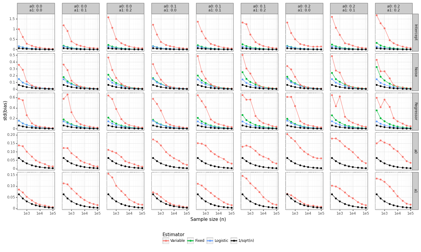
Figure 3 below shows that the rate of convergence of the Hausman estimator is well above the lower-bound we expect from maximum likelihood estimators: \(\hat{\beta}-\beta_0 \overset{a}{\sim}N(0,n^{-1})\). When \((\alpha_0, \alpha_1)\) are fixed, the convergence rate approximates that naive logistic regression model. When there is no label flipping in the DGP \((\alpha_0=0, \alpha_1=0)\), then it takes around 10K samples for the Fixed/Logistic models to achieve root-n convergence. When \((\alpha_0, \alpha_1)\) are estimated by the model, the rate of convergence is even slower, and at least 100K observations are needed for the Variable approach to begin to converge.
Figure 3: Rate of convergence
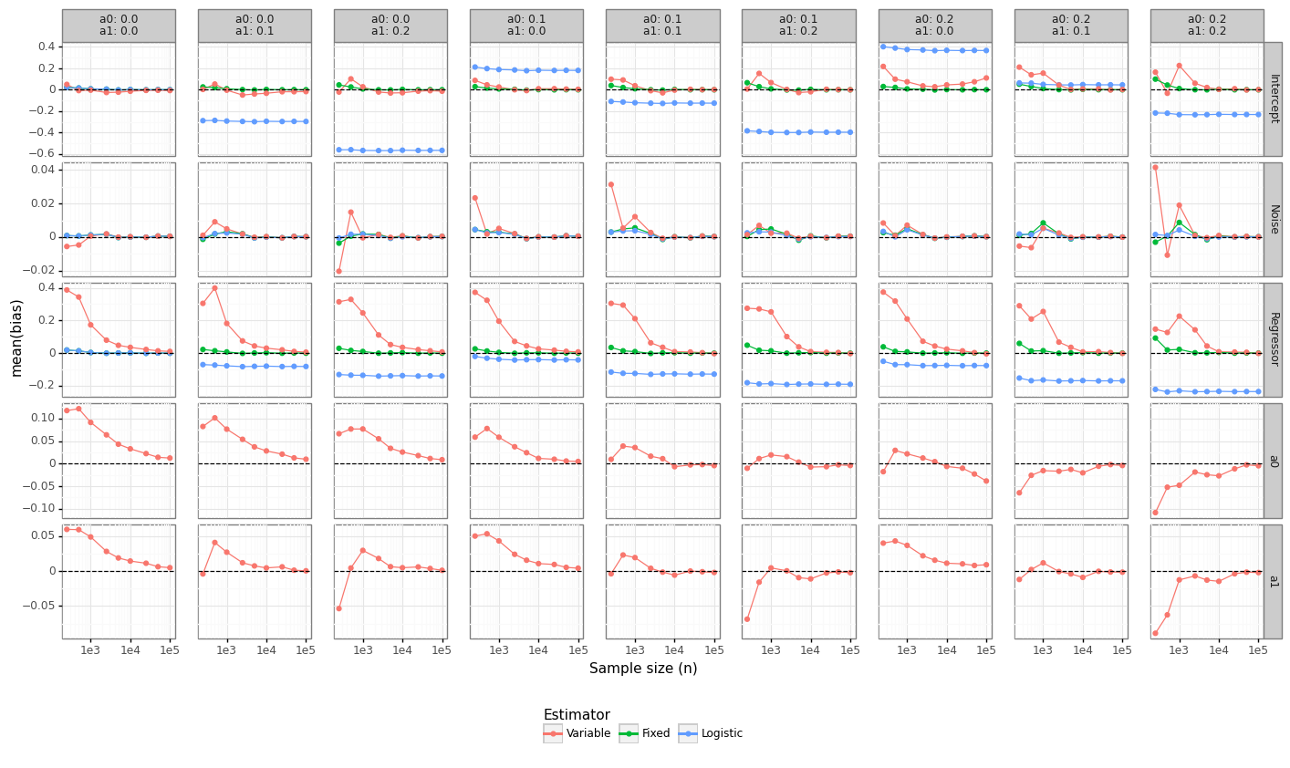
While convergence rates provide insight into the statistical efficiency of an estimator, it does not reveal how far off the average estimate is from its true value. Figure 4 shows that for non-zero label flipping properties, the naive logistic regression model remains permanently biased, regardless of the sample size. When the estimator fixes the values of \((\alpha_0, \alpha_1)\) to the true value, the bias for all coefficients disappears quickly. For the Variable model, the bias on the intercept is killed quickly, whereas the regressor coefficients require at least 10K samples before they become effectively unbiased. Interestingly, while the bias of the Logistic model is negative (which is as expected given that label noise leads to coefficient attenuation), the bias for the Variable model is positive for smaller samples. Since the most important parameter for calibrating a model’s threshold is its intercept, this suggests the Variable model might be able to provide guidance on the true baseline risk.
Figure 4: Parameter bias
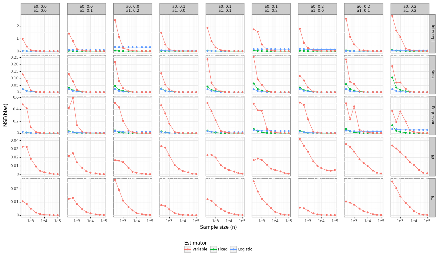
Unbiased models do not necessarily perform better than biased ones when making predictions due to the bias-variance trade-off. Since the underlying DGP is linear, the MSE of the coefficients provides a good approximation for which model will do the best for prediction-type problems. Figure 5 shows that the Fixed estimator dominates in MSE terms (although this is to be expected because it knows the true value of \((\alpha_0,\alpha_1)\)). For the regressor coefficients, the Variable model will begin to outperform the naive logistic regression somewhere between 1-10K observations. This also implies that there exists some imprecise estimate of \((\alpha_0,\alpha_1)\) that when plugged into the estimator and fixed would still outperform either approach.
Figure 5: Parameter MSE
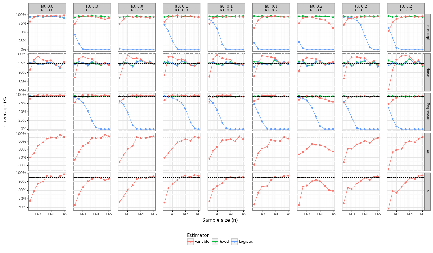
Lastly, we can see whether the standard errors obtained from the inverse of the Hessian provide reasonable coverage properties. Figure 6 shows the coverage for the 95% confidence intervals for the parameter types. For more than 1K observations, the coverage is fairly close to the expected level for the Variable model, although not always. The standard errors for the intercept and the \((\alpha_0,\alpha_1)\) do not appear to be converging even for the large sample size case. The Logistic model’s coverage collapses to zero since the standard errors are shrinking but the bias remains constant.
Figure 6: Coverage properties
(6) Conclusion
This post has shown how to estimate a logistic-type model in the presence of label error when the outcome is binary. Hausman’s proposed modification to likelihood is an intuitive and easy framework that can be used as a loss function in a variety of settings. For example, it can adapted for a deep learning framework:
\[\begin{align*} P(y_i=1 | x_i) &= \alpha_0 + (1-\alpha_0-\alpha_1) F(x_i;\theta), \end{align*}\]Where \(\theta\) are the parameters of the network. I have implemented the functions found in the LogisticHausman class using automatic differentiation here, with gradient checks showing they are highly precise. One could also use this loss function for other techniques like gradient boosting. A further application of the Hausman-logistic loss function is to apply it to machine learning models in a continuous learning setting where feedback loops will cause some of the labels to be mismeasured.
The simulation results shown in section 5 reveal there is a high cost in allowing the model to estimate \((\alpha_0, \alpha_1)\) in terms of convergence rates and mean-squared error. It is possible a naive logistic regression model would outperform the Variable model in terms of accuracy when the sample size is small even though its coefficients would be biased. When a statistical estimate of \((\alpha_0, \alpha_1)\) exists, these can either be plugged in as fixed values, or can inform the bounds applied to the minimization problem. The choice of whether to fix or constrain these parameters will be related to the magnitude of the bias-variance trade-off. The optimal choice will ultimately depend on whether the final goal is parameter inference, prediction, or both. Further experimentation into alternative data generating processes, high dimensional data, and more generic machine learning models would be areas of useful research.
Notes
-
For example, genetic data will have measurement error because variant calling is not 100% accurate. Most socioeconomic data is self-reported (income, ethnicity, etc) which obviously introduces noise. Most medical records will have errors either because the fields are patient reported or it relies on doctors to accurately record the information. ↩
-
It would be interesting to show a proof that the z-score distribution is always conservative (i.e. the rate of change of the coefficients towards zero is faster than the rate of attenuation in the standard errors towards zero). ↩
-
Remember these conclusions rely on the assumption of classical measurement error which is uncorrelated between columns or the response. In reality, most measurement error will actually be generated by a much more complex process whose consequence could be deleterious. ↩