Background

The superior prediction accuracy that machine learning (ML) models tend to have over traditional statistical approaches is largely driven by:

1. Selecting parameter weights for prediction accuracy rather than statistical inference, and
2. Accounting for the tension between in- and out-of-sample accuracy

Many ML are overdetermined in that it is easy for them to completly “master” any training data set they are given by overfitting the data. This leads to poor generalization accuracy because parameter weights are trained on noise which fails to extrapolate to new observations. Therefore models are regularized to prevent them from over-fitting. The intensity of regularization is usually governed by hyperparameters, which are themselves tuned via cross-validation (CV) or risk estimators such as AIC, BIC, or SURE. While statisticians may be more likely to use risk estimators over computer scientists, CV is by far the most common approach today.

What form can hyperparameters take? They range from weights which determine the balance between the \(\ell_1\) and \(\ell_2\) coefficient budget size and training loss in penalized regression to the bandwidth employed by a kernel regression. When a model has a single hyperparameter, a simple line search over a range of values can be performed, where each value of the hyperparameter is given a validation score as measured by a hold-out sample or CV. Below is the pipeline that will often be employed by a ML researcher to train a model for prediction tasks, where \(\bbeta\) is the parameter weights, \(\by\) is the response measures, \(\bX\) is the design matrix, \(\mathcal{L}\) is the loss function, \(P()\) is some penalty measure against overfitting, and \(\lambda\) is the hyperparameter.

• Step 1: Pick a value for \(\lambda\) and solve the constrained minization problem on the training (R) data

• Step 2: Evaluate the model on the test (T) data: \(\LT(\bbetahl,\bX_T,\by_T)\)

• Step 3: Do a line search across a range of \(\lambda\)’s \(\mathcal{D}=\{\lambda_1,\dots,\lambda_m \}\) and find the value that minimizes the test error

In the steps above I omitted the details of the inner loop that Steps 1-2 have with CV as well as and that \(\lambda\) can be a vector, but the same principle applies. Notice that \(\bbetahl\) is indexed by \(\lambda\), because for a given value of the hyperparameter, \(\bbetahl\) has a unique solution.

As the number of hyperparameters increases, line/grid search becomes costly. For example, searching over 100 values of \(\lambda\) and \(\alpha\) for the hyperparameters of the Elastic Net algorithm whilst using 10-fold cross validation requires estimating 100,000 models. Even though this algorithm has a lightning fast convex optimization procedure, searching across the hyperparameter space neither scales well nor lends itself to more complex models.

In addition to grid search (described above) or random search (as the name implies), gradient-based optimization[¹] can also be used. In a future post I’ll summarize some of the work that has already been done which can be implemented on a broader scale, but I wanted to review some first principles in this post and show how this can be done for ridge regression due to the unique properties of the estimator. As in the above pipeline we’ll assume there’s a training and a test set, but the underlying principle can be applied to both CV or risk estimators.

Nested optimization

The bi-level optimization problem can be formulated as follows:

Or alternatively:

Equation \eqref{eq:minmin} looks somewhat odd as there is an \(\arg \min\) inside the function we are trying to minimize. All it means is that \(\bbetah\) will get passed to \(\LT(\cdot)\) and that it is a function of the outer optimization parameter \(\bbetah(\lambda)\), where \(\bbetah\) is the solution to \(\frac{\partial}{\bbeta}\Bigg( \LR + P(\lambda,\bbeta) \Bigg)=\mathbf{0}\).

Example: ridge regression

Because any value of \(\lambda\) is awarded a unique \(\bbetah\), to be able to minimize equation \eqref{eq:bi1} we need to solve:

Equation \eqref{eq:deriv} has a nice interpration: a change in \(\lambda\) first causes a change in \(\bbetah\) which then causes a change in the fitted value and hence prediction loss. The first term in the chain rule can be easy to determine (depends on the loss function), whereas the second term \(\partial \bbetah / \partial \lambda\) is non-trivial as we need the figure out the relationship between how a change in \(\lambda\) changes the coefficients weights to the penalized regression problem. Luckily in the case of ridge regression, this derivative can be analytically derived.

The loss function has taken the form of the sum-of-squares with the fitted values taking a linear form (weighted by \(\bbeta\)), and the penalty term is the \(\ell_2\) norm of the coefficients weighted by \(\lambda\). Ridge regression is one of the few ML estimators that has a closed-form solution,[²] revealing the direct link between \(\lambda\) and its solution.

It will be useful to do a SVD decomposition of \(\bX = \bU \bD \bV^T\) to make the partial derivative easier to calculate.

Where the ridge solution can be formulated to either the OLS coefficient vector (if the solution exists) or the non-diagonal matrices of the SVD. Let’s test this in R to make sure.

# DGP
ss <- 1
set.seed(ss)
N <- 1000
p <- 50
beta <- abs(rnorm(p))
u <- rnorm(N,sd=4)
X <- matrix(rnorm(N * p),nrow=N,ncol=p)
y <- as.vector( (X %*% beta) + u )
# Linear regression
beta.ols <- lm(y ~ -1+X)$coef
# Ridge regresion
library(glmnet)
lam <- 20
beta.ridge.glmnet <- as.vector(coef(glmnet(x=X,y=y,lambda=lam/N,alpha=0,intercept = F,standardize = F))[-1])
# SVD
Xsvd <- svd(X)
U <- Xsvd$u
V <- Xsvd$v
D <- Xsvd$d
# Check
beta.ridge1 <- solve(t(X) %*% X + lam*diag(rep(1,p))) %*% t(X) %*% y
beta.ridge2 <- V %*% diag(D^2 / (lam + D^2)) %*% t(V) %*% beta.ols
beta.ridge3 <- V %*% diag(D / (lam + D^2)) %*% t(U) %*% y
# Close enough
round(head(data.frame(glmnet=beta.ridge.glmnet,approach1=beta.ridge1,
           approach2=beta.ridge2,approach3=beta.ridge3),8),digits=2)

##   glmnet approach1 approach2 approach3
## 1   0.68      0.67      0.67      0.67
## 2   0.45      0.44      0.44      0.44
## 3   0.90      0.89      0.89      0.89
## 4   1.49      1.46      1.46      1.46
## 5   0.21      0.21      0.21      0.21
## 6   0.78      0.77      0.77      0.77
## 7   0.51      0.50      0.50      0.50
## 8   0.81      0.80      0.80      0.80

As long as \(N \gg p\) (so that we can use \(\bbetah^{\text{ols}}\))[³] the derivative from equation \eqref{eq:deriv} for the ridge estimator becomes:

We can now plug in the analytical solution for equation \eqref{eq:deriv} for the ridge regression estimator.

While equation \eqref{eq:ridge_deriv} cannot be solved in closed form, it’s easy enough to write a gradient descent procedure to solve for \(\hlam\).

There are several methods to pick the step-size \(\gamk\), but I will just rely on the Backtracking-line search.

Let’s write some R code and solve for \(\hlam\) after splitting the data into a training and test set.

# Split the data (75/25)
set.seed(ss)
idx.train <- sample(1:nrow(X),floor(nrow(X)*0.75))
idx.test <- setdiff(seq_along(y),idx.train)
y.train <- y[idx.train]
y.test <- y[idx.test]
X.train <- X[idx.train,]
X.test <- X[idx.test,]
# Perform SVD on traning
X.train.svd <- svd(X.train)
U.train <- X.train.svd$u
V.train <- X.train.svd$v
D.train <- X.train.svd$d
# OLS from training
b.ols.T <- as.vector(lm(y.train ~ -1+X.train)$coef)
 
# Function to define ridge regression estimate
fn.beta.ridge <- function(lam,V,D,bols) {
  bridge <- V %*% diag(D^2 / (lam + D^2)) %*% t(V) %*% bols
  return(as.vector(bridge))
}
 
# Define dL/lam=(dL/dbeta) * (dbeta/dlam)
fn.deriv <- function(lam,bridge,yT,XT,VR,DR,bols) {
  # dL/dbeta: Prediction error
  dLdb <- t(t(XT) %*% (yT - as.vector( XT %*% bridge) ))
  # dbeta/dlam
  dbdl <- VR %*% diag(DR^2/(lam+DR^2)^2 ) %*% t(VR) %*% bols
  # Product
  deriv <- as.numeric(dLdb %*% dbdl)
  return(deriv)
}
 
# Function to define generalization loss
fn.loss <- function(yT,XT,bridge) {
  ssL <- 0.5 * sum(as.vector(yT - (XT %*% bridge ))^2)
  return( ssL )
}
 
# --- Run gradient descent --- #
tol <- 10e-8
# Initialize
lam.k0 <- 0
bridge0 <- fn.beta.ridge(lam=lam.k0,V=V.train,D=D.train,bols=b.ols.T)
LT.k0 <- fn.deriv(lam=lam.k0,bridge=bridge0,yT=y.test,XT=X.test,VR=V.train,DR=D.train,
                  bols=b.ols.T)
gamk <- runif(1)
lam.k1 <- lam.k0 - gamk * LT.k0
nsim <- 100
alpha <- 0.5
lam.store <- NULL
i=0
while ((lam.k1-lam.k0)^2 > tol) {
  i=i+1
  # Update
  lam.k0 <- lam.k1
  bridge0 <- fn.beta.ridge(lam=lam.k0,V=V.train,D=D.train,bols=b.ols.T)
  LT.k0 <- fn.deriv(lam=lam.k0,bridge=bridge0,yT=y.test,XT=X.test,VR=V.train,DR=D.train,
                  bols=b.ols.T)
  # Step size
  cond <- T
  gamk <- 100
  while (cond) {
    cond1 <- fn.loss(y.test,X.test,fn.beta.ridge(lam.k0 - gamk * LT.k0,V.train,D.train,b.ols.T))
    cond2 <- fn.loss(y.test,X.test,fn.beta.ridge(lam.k0,V.train,D.train,b.ols.T))
    if (cond1 > cond2) {
      gamk <- gamk * alpha
    } else {
      cond <- F
      lam.k1 <- lam.k0 - gamk * LT.k0
    }
  }
  # Store
  lam.store[i] <- lam.k1
}
print(sprintf('Gradient descent took %i steps',i))

## [1] "Gradient descent took 9 steps"

lam.hat <- lam.store[length(lam.store)]
print(sprintf('Lambda hat is: %0.2f',lam.hat))

## [1] "Lambda hat is: 40.06"

Now that we have our \(\hlam\), we can check that this aligns with the minimum point for test set loss.

# Range of lambdas
lam.seq <- seq(0,100,1)
# Range of beta.hat ridges
beta.seq <- lapply(lam.seq,function(ll) fn.beta.ridge(ll,V=V.train,D=D.train,bols=b.ols.T) )
loss.seq <- lapply(beta.seq,function(bb) fn.loss(y.test,X.test,bb) )
# Plot
plot(lam.seq,loss.seq,
     cex.lab=0.75,cex.axis=0.75,cex.sub=0.75,cex.main=1,
     xlab = expression(lambda),
     ylab='Test set loss',
     main=expression('Relationship of ' * lambda * ' to ' * L[T](lambda)),
     sub=expression('Vertical red line shows ' * lambda * ' found via gradient descent'))
abline(v=lam.hat,col='red')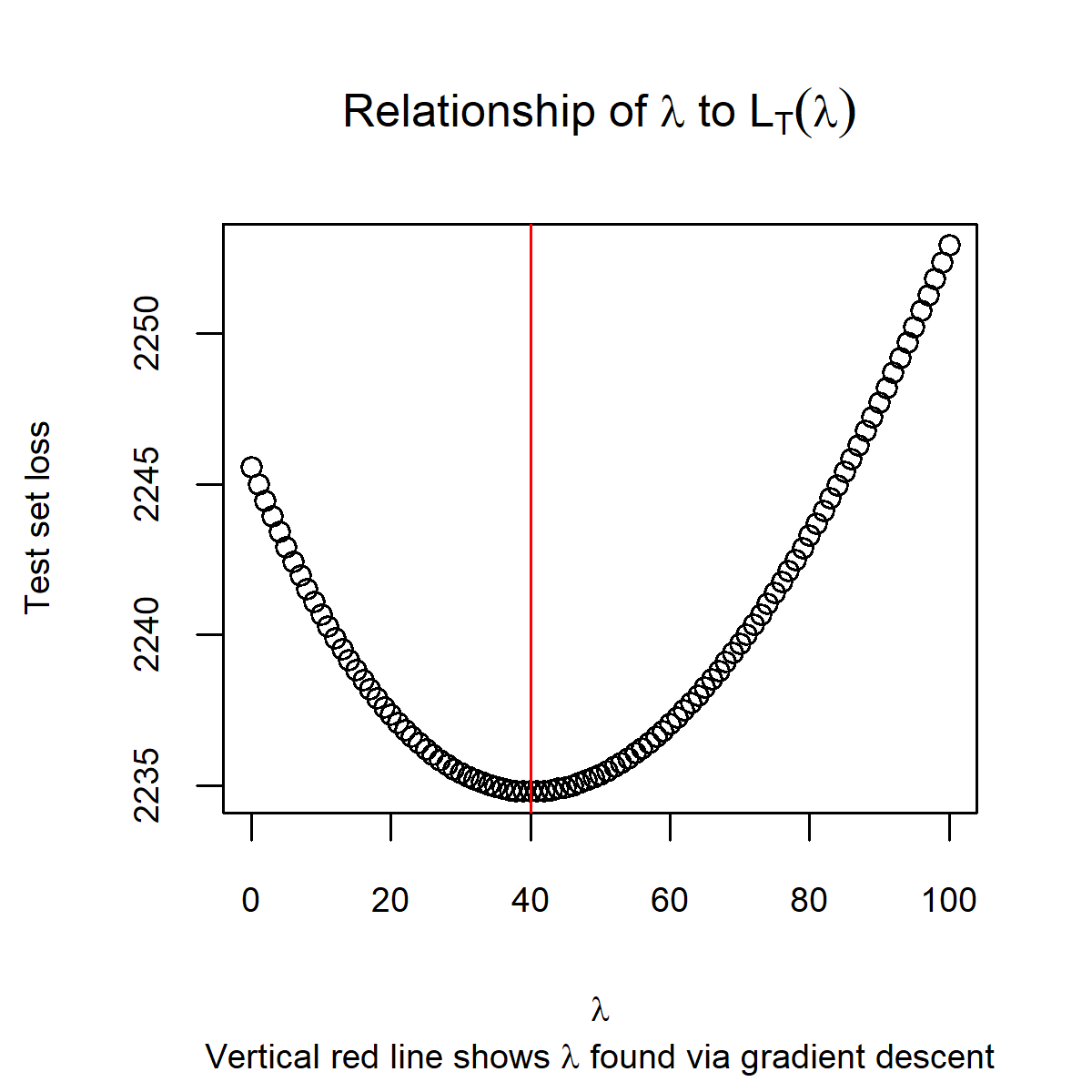

Conclusion

The post has shown that if the derivative of coefficient vector from the inner optimization problem can be derived, one does not need to line/grid search across the held-out data set to determine which \(\lambda\) will minimize the squared error loss. One caveat to this is that the relationship between the hyperparameter and the coefficient weights is smooth, and to ensure a global minimum it must also be convex. Furthermore, this technique is not needed for ridge regression because a line search across \(\lambda\)’s is trivial to perform. In future posts I’ll try to show how this principle can be extended to inexact gradients and the use of multiple hyperparameters.

References

1. Bayesian optimization with scikit-learn

2. Hyperparameter optimization with approximate gradient or this one

3. Gradient-based hyperparameter optimization and the implicit function theorem

4. Truncated Bi-Level Optimization

Footnotes