
Logistic regression from A to Z
Logistic regression (LR) is a type of classification model that is able to predict discrete or qualitative response categories. While LR usually refers to the two-class case (binary LR) it can also generalize to a multiclass system (multinomial LR) or the category-ordered situation (ordinal LR)[1]. By using a logit link, LR is able to map a linear combination of features to the log-odds of a categorical event. While linear models are unrealistic in a certain sense, they nevertheless remain popular due their flexibility and simplicity. LR is commonly used for classification problems in small- to medium-sized data sets despite the bevy of new statistical approaches that have been developed over the past two decades. The development of regularization techniques for LR, including stochastic gradient descent and LASSO, have also helped to maintain LR’s place in the machine learning (ML) model repertoire. While LR is no longer considered “state of the art”, it is worth discussing in detail as it will remain an important approach for developing statistical intuition for aspiring ML practitioners.
The rest of the post will proceed with the following sections: (1) the notation and mathematical foundation of LR models, (2) the classical estimation procedure, (3) analysis of a real-world data set with LR, (4) alternative estimation procedures, (5) the multinomial LR case, and (6) a conclusion and discussion of other issues in LR.
(1) Notational overview[2]
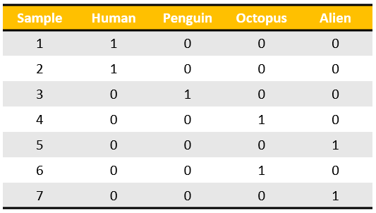
Logistic regression (LR) models a function of the probability of \(K\) discrete classes with a linear combination of \(p\) or \(p+1\) features \(x=(x_1,\dots,x_p)^T\) or \(x=(1,x_1,\dots,x_p)^T\)[3]. When the response (or dependent) variable is discrete and categorical, the prediction task is referred to as classification (as opposed to regression which has a numerical and continuous response). One approach to performing classification is to use a linear regression model but encode the response variable as a matrix in the one-hot encoding format (dimension \(N \times K\)), and then estimate \(K \times p\) coefficients. For a given vector \(x\), classification is done according to which ever fitted value (there will be \(K\) of them) is the largest. There are two issues with this approach: first, some classes may never be predicted (a problem known as masking) and second, the fitted values do not align with intuitions about probability[4].
Figure 1: The one-hot-encoding format
Unlike linear regression, LR ensures that the fitted values are bounded between \([0,1]\), as the log-odds form of the model allows for a mapping to the sigmoid function for the probability values. Notationally, the form of the multinomial logistic regression model is shown below where \(\beta_i^T=(\beta_{i1},\dots,\beta_{ip})\).
\[\begin{align*} \log\frac{P(G=1|X=x)}{P(G=K|X=x)} &= \beta_{10} + \beta_1^T x \\ \vdots \\ \log\frac{P(G=K-1|X=x)}{P(G=K|X=x)} &= \beta_{(K-1)0} + \beta_{K-1}^T x \end{align*}\]For the \(i^{th}\) equation, the dependent variable is the log of the probability of class \(i\) relative to class \(K\) (i.e. the odds), conditional on some feature vector \(x\). Since both an odds and a log transformation are monotonic, the probability of the \(i^{th}\) class can always be recovered from the log-odds. While class \(K\) is used in the denominator above, using the final encoded class is arbitrary, and the the estimated coefficients are equivariant under this choice. While there are \(\frac{K!}{2!(K-2)!}\) relationships in a \(K\)-class LR model[5], only \(K-1\) equations are actually needed. For example, in the \(K=3\) situation, it is easy to see that the log-odds relationship between classes 1 & 2 can be recovered from the log-odds relationship of classes 1 & 3 and 2 & 3.
\[\begin{align*} \frac{\log p_1}{\log p_2} &= (\beta_{10} - \beta_{20}) + (\beta_{1} - \beta_{2})^T x \\ \frac{\log p_1}{\log p_2} &= \gamma_{10} + \gamma_{1}^T x \end{align*}\]Having one less equation than classes ensures that the probabilities sum to one, as the probability of the \(K^{th}\) class is defined as: \(P(G=K|X=x)=1-\sum_{l=1}^{K-1} P(G=l|X=x)\). In the multinomial setting, the parameter \(\theta\) will be used to show that there are actually \((K-1) \times p\) parameters: \(\theta=(\beta_{10},\beta_1^T,\dots,\beta_{(K-1)0},\beta_{K-1}^T )\) that define the system. To save on space, the conditional likelihood may also be denoted as: \(p_k(x;\theta)=P(G=k|X=x)\). After solving the log-odds equations, the probability of each class is:
\[\begin{align*} p_k(x;\theta) &= \frac{\exp(\beta_{k0}+\beta_k^Tx)}{1+\sum_{l=1}^{K-1}\exp(\beta_{l0}+\beta_{l}^Tx)} \hspace{1cm} k=1,\dots,K-1 \\ p_K(x;\theta) &= \frac{1}{1+\sum_{l=1}^{K-1}\exp(\beta_{l0}+\beta_{l}^Tx)} \end{align*}\]In the \(K=2\) situation, the above equations result in the well known sigmoid function: \(p=[1+e^{-(\beta^T x)}]^{-1}\). In classification problems, the function which is used to make the classification choice is referred to as the discriminant function \(\delta\), and it can only be a function of the data. For LR, \(\delta_k(x) = p_k(x;\hat{\theta})\), where the discriminant problem is \(\underset{i}{\text{arg}\max} \hspace{2mm} \delta_i(x), \hspace{2mm} i = 1,\dots,K\). When there are no higher order terms of the features (such as \(x_{i1}^2\)), the LR classification decision boundary is linear.
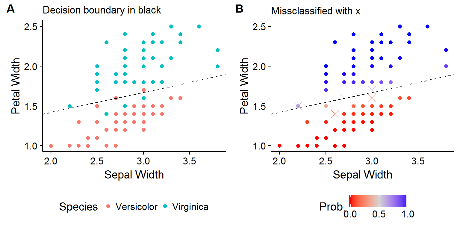
For an example, the Iris data set is considered, where the classification problem is determining whether a flower is of the Versicolor or Virginica species using information regarding petal and sepal width. Figure 2A shows the linear decision boundary using the estimated coefficients. For the two class case it is easy to see that the decision boundary occurs where \(\hat{\beta}^T x > 0\). At the decision boundary, the fitted probabilities are exactly one-half and therefore the flower is classified as the Versicolor species whenever the estimated probability is greater than \(1/2\).
Figure 2: Using LR for flower classification
(2) The classical approach to estimating LR coefficients
The parameters of a LR model, \(\theta\), are estimated by the maximum likelihood approach. For the two-class (binary) case, \(\theta=\beta=\{\beta_{10},\beta_1\}\), and the probability of class \(K=2\) in the denominator can be represented by one less the probability of the first class. Given a data set with a sample of \(N\) independent observations and a vector of inputs \(x_i\) (which includes an intercept), the equation for each observation is:
\[\begin{align*} \log\Bigg(\frac{p(x_i;\beta)}{1-p(x_i;\beta)}\Bigg) &= \beta^Tx_i \hspace{1cm} i=1,\dots,N \end{align*}\]To simplify computations, data are assumed to aggregated so that each observation is a distinct “population”, with \(m_i\) observations associated with a population and \(y_i\) “successes” (the binomial count for each population)[6]. If \(y_i \in \{0,1\} \hspace{2mm} \forall i\) then no observations are aggregated, which is the case for most ML data sets. This leads to following a joint binomial pmf:
\[f(\boldsymbol y|\beta) = \prod_{i=1}^N p(x_i;\beta)^{y_i}(1-p(x_i;\beta))^{1 - y_i}\]Conditioning on a given realization of the data and then expressing the joint distribution as a function of the parameters leads to the likelihood function. Taking the log of this function yields the log-likelihood function, and finding the vector \(\beta\) which maximizes the log-likelihood function will also maximize the likelihood function since a log-transformation is monotonic[7]. Equation \(\eqref{eq:ll}\) shows that the log-likelihood is a non-linear function for each parameter in \(\beta\). Numerical methods will therefore be needed to find the vector \(\beta\) which maximizes the function.
\[\begin{align} l(\beta|\textbf{y}) &= \log L(\beta|\textbf{y}) \nonumber \\ &= \sum_{i=1}^N \Big\{ y_i \log [p(x_i;\beta)] + (1-y_i) \log [1-p(x_i;\beta)] \Big\} \nonumber \\ &= \sum_{i=1}^N \Big\{ y_i [\beta^T x_i] - \log [1+\exp\{\beta^Tx_i \}] \Big\} \tag{1}\label{eq:ll} \end{align}\]The classical approach for multivariate numerical estimation relies on the gradient (or score vector) and hessian (or information matrix) of the log-likelihood function. The former is a vector of partial derivatives and latter is a matrix of all second-order partial derivatives. The \(j^{th}\) and \(jk^{th}\) element of the gradient and hessian are shown in equations \(\eqref{eq:scorej}\) and \(\eqref{eq:hessjk}\), respectively.
\[\begin{align} [S(\beta)]_j &= \frac{\partial l(\beta|\textbf{y})}{\partial \beta_j} \nonumber \\ &= \sum_{i=1}^N \Bigg[ \Bigg(y_i - \overbrace{\frac{\exp\{\beta^Tx_i \}}{1+\exp\{\beta^Tx_i \}}}^{p(x_i;\beta)}\Bigg)x_{ij} \Bigg] \tag{2}\label{eq:scorej} \\ [H(\beta)]_{jk} &= \frac{\partial^2l(\beta|\textbf{y})}{\partial \beta_j\partial \beta_k} \nonumber \\ &= - \sum_{i=1}^N \overbrace{\frac{\exp\{\beta^Tx_i \}}{1+\exp\{\beta^Tx_i \}}}^{p(x_i;\beta)} \overbrace{\frac{1}{1+\exp\{\beta^Tx_i \}}}^{1-p(x_i;\beta)} x_{ij}x_{ik} \tag{3}\label{eq:hessjk} \end{align}\]In order to simplify some of the subsequent stages, it is useful to be able to write the score and hessian in matrix notation. The following notation will aid in the endeavor:
\[\begin{align*} \mathbf{X} &= [\mathbf{1} \hspace{2mm} X_1 \hspace{2mm} \dots \hspace{2mm} X_p] \\ \mathbf{y} &= [y_1,\dots,y_N]^T \\ \mathbf{p} &= [p(x_1;\beta),\dots,p(x_N;\beta)]^T \\ \mathbf{W} &= \text{diag}[p(x_1;\beta)(1-p(x_1;\beta)),\dots,p(x_N;\beta)(1-p(x_N;\beta))] \\ \end{align*}\]This allows the score vector to be written as:
\[\begin{align} [S(\beta)]_j &= \sum_{i=1}^N \{ [y_i - p(x_i;\beta)]x_{ij} \} \nonumber \\ &= \mathbf{X}_j^T[\mathbf{y}-\mathbf{p}] \nonumber \\ S(\beta) &= \mathbf{X}^T[\mathbf{y}-\mathbf{p}] \tag{4}\label{eq:score} \end{align}\]Similarly for the Hessian:
\[\begin{align} [H(\beta)]_{jk} &= - \sum_{i=1}^N \Big[ p(x_i;\beta) (1-p(x_i;\beta)) x_{ij}x_{ik} \Big] \nonumber \\ &= - \begin{bmatrix} x_{1j} & \dots & x_{Nj} \end{bmatrix} \begin{pmatrix} p_1(1-p_1) & & \mathbf{0} \\ & \ddots & \\ \mathbf{0} & & p_N(1-p_N) \end{pmatrix} \begin{bmatrix} x_{1k} \\ \vdots \\ x_{Nk} \end{bmatrix} \nonumber \\ &= - \mathbf{X}_j^T \mathbf{W} \mathbf{X}_k \nonumber \\ H(\beta) &= - \mathbf{X}^T \mathbf{W} \mathbf{X} \tag{5}\label{eq:hess} \end{align}\]The ML estimate \(\hat{\beta}\) is found where \(\partial l(\hat{\beta}|\textbf{y}) / \partial \beta_j =0\) for \(j=0,\dots,p\). Specifically, the classical approach uses Newton-Raphson algorithm to find the ML estimate. This method appeals to the use of a Taylor expansion of the score vector about the point \(\beta_0\) (this is a vector point not a scalar).
\[\begin{align} \nabla l(\beta) &\approx \nabla l(\beta_0) + H(\beta_0) (\beta-\beta_0) = 0 \nonumber \\ \beta &= \beta_0 - [H(\beta_0)]^{-1}\nabla l(\beta_0) \nonumber \\ \beta^{\text{new}} &= \beta^{\text{old}} - [H(\beta^{\text{old}})]^{-1} S(\beta^{\text{old}}) \tag{6}\label{eq:nr} \end{align}\]Using the South African Heart Disease data set (which will be analyzed further in the next section) as an example, the following R code shows how to implement the Newton-Raphson procedure. Note that the update procedure terminates when the euclidean distance between the new and old coefficient vector is less than 0.01.
# Load the data
dat <- ElemStatLearn::SAheart
vo <- c('sbp','tobacco','ldl','famhist','obesity','alcohol','age')
X <- dat[,vo]
# Re-code famhist
X <- cbind(intercept=1,famhist=model.matrix(~-1+famhist,data=dat)[,2],X[,-which(colnames(X)=='famhist')])
X <- as.matrix(X)[,c('intercept',vo)]
y <- dat$chd
# Define the p(x_i;beta) function
p <- function(xi,beta) { 1/(1+exp(-(sum(xi*beta)))) }
# Set up optimization parameters
beta.old <- rep(0,ncol(X))
tol <- 10e-3
dist <- 1
i <- 0
# Begin the loop!
while(dist > tol) {
  i <- i + 1
  # Get the p-vector
  p.vec <- apply(X,1,p,beta=beta.old)
  # Get the W weight matrix
  W <- diag(p.vec*(1-p.vec))
  # Get the Score vector (i.e. gradient)
  dldbeta <- t(X) %*% (y-p.vec)
  # Get the Hessian
  dl2dbeta2 <- -t(X) %*% W %*% X
  # Update beta
  beta.new <- beta.old - solve(dl2dbeta2) %*% dldbeta
  # Calculate distance
  dist <- sqrt(sum((beta.new-beta.old)^2))
  # Reset
  beta.old <- beta.new
}
paste('Convergence achieved after',i,'steps',sep=' ')
## [1] "Convergence achieved after 4 steps"round(beta.new,3)## [,1]
## intercept -4.130
## sbp 0.006
## tobacco 0.080
## ldl 0.185
## famhist 0.939
## obesity -0.035
## alcohol 0.001
## age 0.043An alternative approach which yields identical results is to substitute in \(\eqref{eq:score}\) and \(\eqref{eq:hess}\) into \(\eqref{eq:nr}\) and then re-define some terms to get the “iteratively reweighted least squares” (IRLS) algorithm. Equation \(\eqref{eq:irls}\) shows that at each step of the IRLS, the new vector is the solution to the weighted OLS regression on the adjusted response vector \(\mathbf{z}\). It is easy to show that show that equation \(\eqref{eq:irls}\) is equivalent to \(\underset{\beta}{\text{arg}\min} (\mathbf{z}-\mathbf{X}\beta)^T\mathbf{W} (\mathbf{z}-\mathbf{X}\beta)\)
\[\begin{align} \beta^{\text{new}} &= \beta^{\text{old}} + (\mathbf{X}^T\mathbf{W}\mathbf{X})^{-1}\mathbf{X}^T(\mathbf{y}-\mathbf{p}) \nonumber \\ &= (\mathbf{X}^T\mathbf{W}\mathbf{X})^{-1}\mathbf{X}^T \mathbf{W}\mathbf{z} \tag{7}\label{eq:irls} \\ \underset{\text{Adj. resp.}}{\mathbf{z}} &= \mathbf{X}\beta^{\text{old}} + \mathbf{W}^{-1}(\mathbf{y}-\mathbf{p}) \nonumber \end{align}\]The R code implementation for the IRLS algorithm yields the same results, but is notationally more elegant.
# Set up optimization parameters
beta.old <- rep(0,ncol(X))
tol <- 10e-3
dist <- 1
i <- 0
# Begin the loop!
while(dist > tol) {
  i <- i + 1
  # Get the p-vector
  p.vec <- apply(X,1,p,beta=beta.old)
  # Get the W weight matrix
  W <- diag(p.vec*(1-p.vec))
  # Get W inverse
  Winv <- diag(1/(p.vec*(1-p.vec)))
  # Get z
  z <- (X %*% beta.old) + Winv %*% (y-p.vec)
  # Update beta
  beta.new <- solve(t(X) %*% W %*% X) %*% t(X) %*% W %*% z
  # Calculate distance
  dist <- sqrt(sum((beta.new-beta.old)^2))
  # Reset
  beta.old <- beta.new
}
paste('Convergence achieved after',i,'steps',sep=' ')
## [1] "Convergence achieved after 4 steps"round(beta.new,3)## [,1]
## intercept -4.130
## sbp 0.006
## tobacco 0.080
## ldl 0.185
## famhist 0.939
## obesity -0.035
## alcohol 0.001
## age 0.043(3) South African Hearth Disease Data Set
This section will consider how LR can be used to estimate the risk of coronary heart disease (CHD) using the SAheart data set that is part of the ElemStatLearn library as well as how the coefficients of the LR model can be interpreted when performing statistical inference. This data set has \(N=462\) observations for white males (ages 15-64) with a response variable of whether they have a type of coronary heart disease: myocardial infarction (chd) along with seven control variables including systolic blood pressure (sbp), low density lipoprotein cholesterol (ldl), and body fat (adiposity).
##   sbp tobacco  ldl adiposity famhist typea obesity alcohol age chd
## 1 160   12.00 5.73     23.11 Present    49   25.30   97.20  52   1
## 2 144    0.01 4.41     28.61  Absent    55   28.87    2.06  63   1
## 3 118    0.08 3.48     32.28 Present    52   29.14    3.81  46   0
## 4 170    7.50 6.41     38.03 Present    51   31.99   24.26  58   1
Figure 3 shows the correlation matrix of the seven features, with observations color coded for cases and controls of CHD. Clearly no two-pair feature space provides a nice linear discriminant line (compare this to Iris data set seen in the first section).
Figure 3: SA Heart features
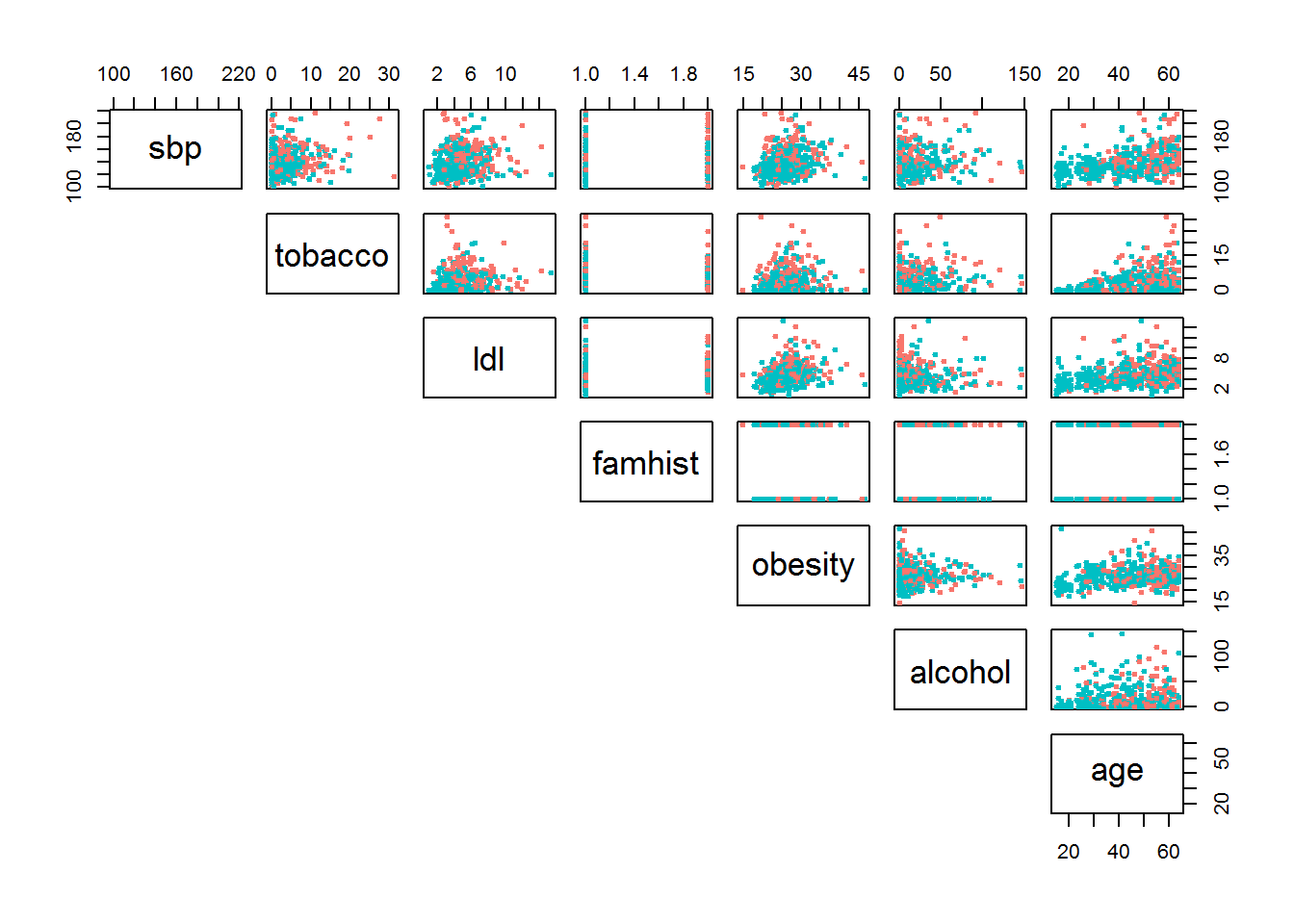
Red is cases and teal is controls
Fitting a LR model is very easy using base R and can be done with the glm function by specifying the correct family option.
glm(chd~sbp+tobacco+ldl+famhist+obesity+alcohol+age,data=dat,family=binomial(link=logit))Table 1A shows the coefficient estimates for the data set using LR with all seven features. Not all the results are intuitive including the fact that the systolic blood pressure variable is insignificant and the coefficient sign suggests that obesity lowers the risk of CHD!
| Estimate | Std. Error | z value | Pr(> | z| ) | |
| (Intercept) | -4.130 | 0.964 | -4.283 | 0.00002 |
| sbp | 0.006 | 0.006 | 1.023 | 0.306 |
| tobacco | 0.080 | 0.026 | 3.034 | 0.002 |
| ldl | 0.185 | 0.057 | 3.219 | 0.001 |
| famhistPresent | 0.939 | 0.225 | 4.177 | 0.00003 |
| obesity | -0.035 | 0.029 | -1.187 | 0.235 |
| alcohol | 0.001 | 0.004 | 0.136 | 0.892 |
| age | 0.043 | 0.010 | 4.181 | 0.00003 |
The insignificant and counter-intuitive results are likely driven by the inclusion of extraneous and multicollinear variables. For small data sets like this one, a backward selection strategy (a specific type of stepwise regression) where variables are iteratively dropped from the model until the AIC stops falling can be used to pare down the model. This is also fairly easy to implement in R by using the step function.
mdl.full <- glm(chd~sbp+tobacco+ldl+famhist+obesity+alcohol+age,data=dat,family=binomial(link=logit))
mdl.bw <- step(mdl.full,direction = 'backward',trace=0)
Three variables are dropped after the backward selection procedure, and the remaining covariates are shown in Table 1B. All four features increase the log-odds of CHD, a result which aligns with our intuition about the relationship between heart disease and tobacco use, LDL levels, a family history of the disease, and age.
| Estimate | Std. Error | z value | Pr(> | z| ) | |
| (Intercept) | -4.204 | 0.498 | -8.437 | 0 |
| tobacco | 0.081 | 0.026 | 3.163 | 0.002 |
| ldl | 0.168 | 0.054 | 3.093 | 0.002 |
| famhistPresent | 0.924 | 0.223 | 4.141 | 0.00003 |
| age | 0.044 | 0.010 | 4.521 | 0.00001 |
How can one specifically interpret the coefficients from a logistic regression, such as the \(\hat{\beta}_{\text{age}}=0.044\) result from Table 1B? Consider two input vectors \(x_a\) and \(x_b\) that share the same covariate values except that the individual associated with \(x_a\) is one year older. By subtracting the two fitted values, it is easy to see that the difference is equal to \(\hat{\beta}_{\text{age}}\). Therefore, the coefficient results of a LR model should be interpreted as follows: a one unit change in a feature \(j\) leads to a \(\hat{\beta}_j\) increase in the log-odds (also known as the log-odds ratio) of the condition.
\[\begin{align*} x_a &= [1,\text{tobacco}_0,\text{ldl}_0,\text{famhist}_0,\text{age}_0+1]^T \\ x_b &= [1,\text{tobacco}_0,\text{ldl}_0,\text{famhist}_0,\text{age}_0]^T\\ \underbrace{\hat{\beta}^T(x_a - x_b)}_{\hat{\beta}^T [0,0,0,0,1]^T} &= \log\Bigg(\frac{p(x_a;\hat{\beta})}{1-p(x_a;\hat{\beta})}\Bigg) - \log\Bigg(\frac{p(x_a;\hat{\beta})}{1-p(x_a;\hat{\beta})}\Bigg) \\ \hat\beta_{\text{age}} &= \log\Bigg(\frac{p(x_a;\hat{\beta})/(1-p(x_a;\hat{\beta}))}{p(x_b;\hat{\beta})/(1-p(x_b;\hat{\beta}))} \Bigg) \end{align*}\]Alternatively, the natural exponential function evaluated at the coefficient estimate can be interpreted as the increase in the odds of the event.
\[\exp\{\hat\beta_{\text{age}}\} = \frac{p(x_a;\hat{\beta})/(1-p(x_a;\hat{\beta}))}{p(x_b;\hat{\beta})/(1-p(x_b;\hat{\beta}))}\]For this data set, the LR results suggest that becoming one-year older leads to an increase of the odds of coronary heart disease by 1.045. To determine statistical significance, confidence intervals (CI) can be constructed by appealing to the fact that the maximum likelihood estimate is (asymptotically) normal. If the CI for the odds contains “1”, then the result is insignificant.
\[\begin{align*} &(1-\alpha)\% \text{ CI for the change in odds} \\ \exp \Big\{ \hat\beta_{\text{age}} &\pm Z_{1-\alpha/2}\sqrt{\hat{\text{Var}}(\hat\beta_{\text{age}})} \Big\} = \{1.025,1.065 \} \end{align*}\](4) Alternative estimation procedures
LR was developed well before the big data era, when observations tended to number in the hundreds and features in the dozens. The classical estimation approach to LR begins to breakdown when \(p\) grows as finding the inverse of the \(H\) or \(X^T W X\) term for the Newton-Raphson or IRLS algorithm is an \(O(p^3)\) problem. When \(N\) gets very large, calculating the \(\sum_{i=1}^N p(x_i;\beta)\) term can be computationally time consuming too. This section will discuss using the techniques of gradient descent for the large-\(p\) problem and stochastic gradient descent for the large-\(N\) problem.
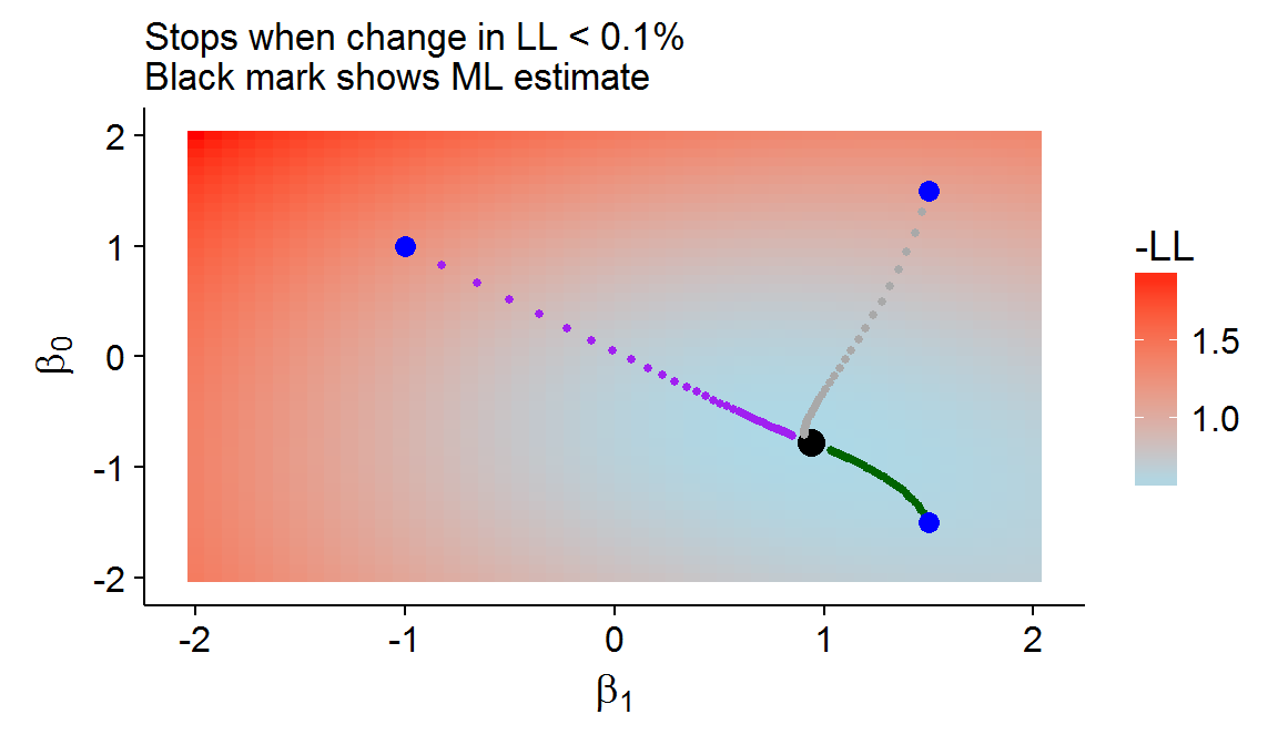
For gradient descent, the Hessian is ignored and some step size \(\eta\) is used to update the Newton-Raphson algorithm: \(\beta^{\text{new}} = \beta^{\text{old}} - \eta \frac{-\partial l(\beta)}{\partial\beta}\). The method is called gradient “descent” because the negative log-likelihood is used so that the score vector points in the direction which minimizes the negative log-likelihood (and maximizes the log-likelihood) function. Gradient descent will generally converge to the global minima when the step size is small enough and the likelihood space is convex (i.e. it looks like a valley). The figure below shows gradient descent with an intercept and the age variable (normalized) from the SA heart data set at various starting points with \(\eta=0.5\). The choice of step size and stopping criterion is akin to selecting hyperparameters for ML algorithms. Data-driven methods like cross-validation will likely select parameters that stop “too soon” for any given realization, but have better generalization performance. In this sense, gradient descent can function as a type of regularization.
Figure 4: An example of gradient descent
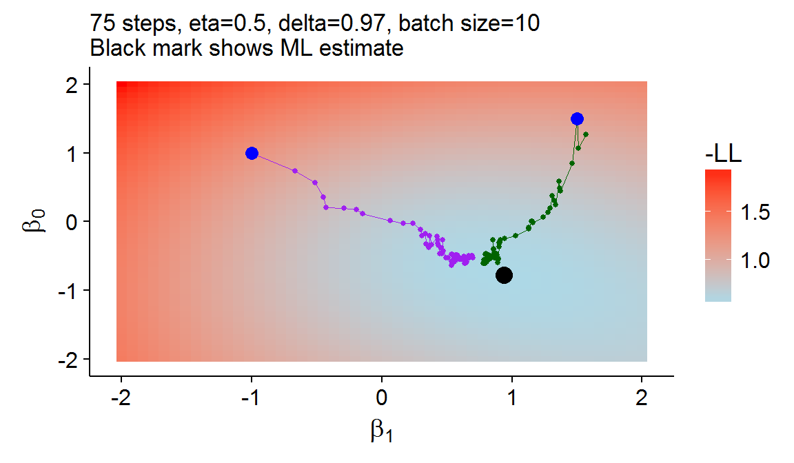
The log-likelihood is always made up of \(N\) “summand functions”: \(\sum_{i=1}^N Q_i\), where \(Q_i=y_i [\beta^T x_i] - \log [1+\exp(\beta^Tx_i)]\) for the binary LR model. With stochastic gradient descent (SGD), only one (or a batch) of these summand functions are (randomly) selected to be used in the update of the gradient descent algorithm. In addition to the initial learning rate, a decay rate must be chosen for SGD so that the step size decreases over time: \(\eta_t=\delta\eta_{t-1}\). Figure 5 shows the SGD approach is able to achieve a similar result to the gradient descent or the classical Newton-Raphson approach but at a much lower computational cost[8].
Figure 5: An example of stochastic gradient descent
(5) Multinomial Logistic Regression
When the number of classes is greater than two, several modifications need to be made to both the likelihood and matrix formulation of the Newton-Raphson estimation procedure. The rest of this section will show the mathematical and matrix calculations needed to handle this slightly more complex LR form. The responses are now one-hot encoded in an \(N \times (K-1)\) matrix, \(\mathbf{Y}\), whose \(i^{th}\) row, \(\mathbf{y}_i\), is a \(K-1\) row vector, whose \(j^{th}\) element is only equal to one if it belongs to class \(j\).
\[\begin{align*} \mathbf{Y} &= \begin{pmatrix} \mathbf{y}_1 \\ \vdots \\ \mathbf{y}_N \end{pmatrix} = \begin{pmatrix} (y_{11}, \hspace{2mm} \dots \hspace{2mm} y_{1(K-1)} \\ \vdots \\ (y_{N1}, \hspace{2mm} \dots \hspace{2mm} y_{N(K-1)} ) \end{pmatrix} \end{align*}\]The joint pmf becomes the multinomial rather than the binomial distribution, whose \(i^{th}\) contribution to the product of terms is shown below.
\[\begin{align*} p_{\mathbf{y}_i}(x_i) &= P(G=1|X=x_i)^{y_{i1}} \times \cdots \times P(G=K-1|X=x_i)^{y_{i(K-1)}}\times P(G=K|X=x_i)^{1-\sum_{l=1}^{K-1} y_{il}} \end{align*}\]Hence, the \(i^{th}\) summand of the log-likelihood is going to be:
\[\begin{align*} \log(p_{\mathbf{y}_i}(x_i)) &= y_{i1}\log P(G=1|X=x_i) + \cdots + \\ & y_{i(K-1)}\log P(G=K-1|X=x_i) + (1-\sum_{l=1}^{K-1} y_{il}) \log P(G=K|X=x_i) \\ &= \log P(G=K|X = x_i) + \sum_{l=1}^{K-1} \log \frac{P(G=l|X=x_i)}{P(G=K|X=x_i)} \\ &= \log P(G=K|X = x_i) + \sum_{l=1}^{K-1} [\beta_l^T x_i]y_{il} \\ l(\theta|\mathbf{Y}) &= \sum_{i=1}^N \Bigg[\sum_{l=1}^{K-1} [\beta_l^T x_i]y_{il} + \log P(G=K|X = x_i) \Bigg] \\ &= \log P(G=K|X = x_i) + \sum_{l=1}^{K-1} [\beta_l^T x_i]y_{il} \\ &= \sum_{i=1}^N \Bigg[\sum_{l=1}^{K-1} [\beta_l^T x_i]y_{il} - \log \Bigg(1 + \sum_{l=1}^{K-1} \exp\{\beta_l^T x_i \} \Bigg) \Bigg] \end{align*}\]To actually estimate the parameters, it will be useful to vertically “stack” all the observations and parameters. There will be \(K-1\) vertical blocks of \(p+1\) parameters for the different classes.
\[\begin{align*} \underbrace{\theta}_{(K-1)(p+1)\times 1} &= \begin{bmatrix} \beta_1 \\ \vdots \\ \beta_{K-1}\end{bmatrix} = \begin{bmatrix}\beta_{10} \\ \beta_{11} \\ \beta_{12} \\ \vdots \\ \beta_{(K-1)p}\end{bmatrix} \end{align*}\]Consider the \(p+1\) partial derivatives for the score vector for the \(l^{th}\) block of parameters.
\[\begin{align*} \frac{\partial l(\theta)}{\partial\beta_{l0}} &= \sum_{i=1}^N \Bigg[ y_{il}x_{i0} - \Bigg(\frac{\exp\{\beta^T_l x_i \}}{1+ \sum_{l'=0}^{K-1}\exp\{\beta^T_{l'} x_i \}}\Bigg)x_{i0} \Bigg] \\ &\vdots \\ \frac{\partial l(\theta)}{\partial\beta_{lp}} &= \sum_{i=1}^N \Bigg[ y_{il}x_{ip} - \Bigg(\frac{\exp\{\beta^T_l x_i \}}{1+ \sum_{l'=0}^{K-1}\exp\{\beta^T_{l'} x_i \}}\Bigg)x_{ip} \Bigg] \\ \underbrace{\frac{\partial l(\theta)}{\partial\beta_{l}}}_{(p+1)\times 1} &= \sum_{i=1}^N y_{il}\begin{bmatrix}x_{i0} \\ \vdots \\ x_{ip}\end{bmatrix} - \sum_{i=1}^N P(G=l|X=x_i) \begin{bmatrix}x_{i0} \\ \vdots \\ x_{ip}\end{bmatrix} \\ \frac{\partial l(\theta)}{\partial\beta_{l}} &= \sum_{i=1}^N y_{il}x_i - \sum_{i=1}^N P(G=l|X=x_i)x_i \end{align*}\]Next denote:
\[\begin{align*} \textbf{t}_l &= \begin{bmatrix}y_{1l} \\ \vdots \\ y_{nl} \end{bmatrix} \hspace{1cm} and \hspace{1cm} \textbf{p}_l = \begin{bmatrix}P(G=l|X=x_1) \\ \vdots \\ P(G=l|X=x_n) \end{bmatrix} \\ \mathbf{X}^T \textbf{t}_l &= \begin{pmatrix}x_{10} & \dots & x_{N0} \\ \vdots & & \vdots \\ x_{1p} & \dots & x_{Np} \end{pmatrix} \begin{bmatrix}y_{1l} \\ \vdots \\ y_{nl} \end{bmatrix} = \begin{pmatrix}\sum_{i=1}^N x_{i0}y_{il} \\ \vdots \\ \sum_{i=1}^N x_{ip}y_{il} \end{pmatrix} \\ &= \sum_{i=1}^N y_{il}x_i \\ &\text{Similarly} \\ \mathbf{X}^T \textbf{p}_l &= \sum_{i=1}^N P(G=l|X=x_i)x_i \\ \frac{\partial l(\theta)}{\partial\beta_{l}} &= \mathbf{X}^T (\textbf{t}_l - \textbf{p}_l ) \end{align*}\]The final score vector of length \((p+1)\times (K-1)\) will take the following form:
\[\begin{align*} \frac{\partial l(\theta|\mathbf{Y})}{\partial \theta} &= \underbrace{\begin{bmatrix} \mathbf{X}^T(\textbf{t}_1 - \textbf{p}_1 ) \\ \vdots \\ \mathbf{X}^T(\textbf{t}_{K-1} - \textbf{p}_{K-1} ) \end{bmatrix}}_{(p+1)N \times 1} \\ &= \begin{bmatrix}\mathbf{X}^T & 0 \dots & 0 \\ 0 & \mathbf{X}^T & \dots & 0 \\ \vdots & & \vdots \\ 0 & \dots & \dots & \mathbf{X}^T \end{bmatrix} \begin{bmatrix} \textbf{t}_1 - \textbf{p}_1 \\ \textbf{t}_2 - \textbf{p}_2 \\ \\\vdots \\ \textbf{t}_{K-1} - \textbf{p}_{K-1} \end{bmatrix} \\ &= \underbrace{\tilde{\mathbf{X}}^T}_{(p+1)(K-1)\times N(K-1)} \underbrace{[\tilde{\textbf{t}}-\tilde{\textbf{p}}]}_{N(K-1)\times 1} \end{align*}\]The Hessian for the multinomial LR has the additional wrinkle that the diagonal and off-diagonal blocks will be different. Beginning with the matrices on the diagonals:
\[\begin{align*} \frac{\partial^2l(\theta)}{\partial \beta_l \partial \beta_l^T}\ &= -\sum_{i=1}^N \frac{\partial P(G=l|X=x_i)}{\partial \beta_l^T} x_i \\ \frac{\partial P(G=l|X=x_i)}{\partial \beta_l^T} &= \begin{bmatrix} \frac{\partial}{\partial \beta_{l0} } & \dots & \frac{\partial}{\partial \beta_{lp} }\end{bmatrix} \frac{\exp\{\beta_l^T x_i\}}{1+\sum_{l'=1}^{K-1}\exp\{\beta_{l'}^T x_i\}} \\ &\text{The \\(j^{th}\\) element is going to be:} \\ \Big[\frac{\partial P(G=l|X=x_i)}{\partial \beta_l^T}\Big]_j &= \frac{\exp\{\beta_l^T x_i\}}{1+\sum_{l'=1}^{K-1}\exp\{\beta_{l'}^T x_i\}}x_{ij} - \Bigg(\frac{\exp\{\beta_l^T x_i\}}{1+\sum_{l'=1}^{K-1}\exp\{\beta_{l'}^T x_i\}}\Bigg)^2 x_{ij} \\ \frac{\partial P(G=l|X=x_i)}{\partial \beta_l^T} &= P(G=l|X=x_i)(1-P(G=l|X=x_i)) x_i^T \\ \frac{\partial^2l(\theta)}{\partial \beta_l \partial \beta_l^T}\ &= - \sum_{i=1}^N P(G=l|X=x_i)(1-P(G=l|X=x_i)) x_i x_i^T \end{align*}\]Then for the off diagonals:
\[\begin{align*} \frac{\partial^2l(\theta)}{\partial \beta_l \partial \beta_k^T} &= -\sum_{i=1}^N \frac{\partial P(G=l|X=x_i)}{\partial \beta_k^T} x_i \\ \frac{\partial P(G=l|X=x_i)}{\partial \beta_k^T} &= \begin{bmatrix} \frac{\partial}{\partial \beta_{k0} } & \dots & \frac{\partial}{\partial \beta_{kp} }\end{bmatrix} \frac{\exp\{\beta_l^T x_i\}}{1+\sum_{l'=1}^{K-1}\exp\{\beta_{l'}^T x_i\}} \\ &= \begin{pmatrix}- \frac{\exp\{\beta_l^T x_i\}}{(1+\sum_{l'=1}^{K-1}\exp\{\beta_{l'}^T x_i\})^2}\exp\{\beta_k^Tx_i\}x_{i0} \\ \vdots \\ - \frac{\exp\{\beta_l^T x_i\}}{(1+\sum_{l'=1}^{K-1}\exp\{\beta_{l'}^T x_i\})^2}\exp\{\beta_k^Tx_i\}x_{ip} \end{pmatrix}^T \\ &= - \begin{pmatrix}P(G=l|X=x_i)P(G=k|X=x_i)x_{i0} \\ \vdots \\ P(G=l|X=x_i)P(G=k|X=x_i)x_{ip}\end{pmatrix}^T \\ \frac{\partial^2l(\theta)}{\partial \beta_l \partial \beta_k^T}\ &= \sum_{i=1}^N P(G=l|X=x_i)P(G=k|X=x_i) x_i x_i^T \\ \end{align*}\]The final Hessian will therefore be made up \(K-1 \times K-1\) matrices.
\[\begin{align*} \frac{\partial ^2 l(\theta)}{\partial \theta \partial \theta^T} &= \begin{bmatrix} \frac{\partial^2l(\theta)}{\partial \beta_1 \partial \beta_1^T} & \frac{\partial^2l(\theta)}{\partial \beta_1 \partial \beta_2^T} & \dots & \frac{\partial^2l(\theta)}{\partial \beta_1 \partial \beta_{K-1}^T} \\ & & \vdots & \\ \frac{\partial^2l(\theta)}{\partial \beta_{K-1} \partial \beta_1^T} & \frac{\partial^2l(\theta)}{\partial \beta_{K-1} \partial \beta_2^T} & \dots & \frac{\partial^2l(\theta)}{\partial \beta_{K-1} \partial \beta_{K-1}^T} \end{bmatrix} \end{align*}\]Introducing some further matrix notation:
\[\begin{align*} \mathbf{Q}_l &= \text{diag}[p_l(x_1)(1-p_l(x_1)),\dots,p_l(x_n)(1-p_l(x_n))] \\ \mathbf{R}_l &= \text{diag}[p_l(x_1),\dots,p_l(x_n)] \end{align*}\]This allows the matrix formulation of the Hessian.
\[\begin{align*} \frac{\partial^2l(\theta)}{\partial \beta_l \partial \beta_l^T} &= - \mathbf{X}^T \mathbf{Q}_l \mathbf{X} \\ \frac{\partial^2l(\theta)}{\partial \beta_l \partial \beta_k^T} &= \mathbf{X}^T \mathbf{R}_l \mathbf{R}_k \mathbf{X} \\ \frac{\partial ^2 l(\theta)}{\partial \theta \partial \theta^T} &= -\tilde{\mathbf{X}}^T \begin{bmatrix} \mathbf{Q}_1 & -\mathbf{R}_1\mathbf{R}_2 & \dots & -\mathbf{R}_1\mathbf{R}_{K-1} \\ -\mathbf{R}_2\mathbf{R}_1 & \mathbf{Q}_2 & \dots & -\mathbf{R}_2\mathbf{R}_{K-1} \\ & & \vdots & \\ -\mathbf{R}_{K-1}\mathbf{R}_1 & -\mathbf{R}_{K-1}\mathbf{R}_2 & \dots & \mathbf{Q}_{K-1} \end{bmatrix} \tilde{\mathbf{X}} \\ &= - \tilde{\mathbf{X}}^T \tilde{\mathbf{W}} \tilde{\mathbf{X}} \end{align*}\]Using the terms defined above, the Newton-Raphson algorithm can be written in a very similar form.
\[\begin{align*} \theta^{\text{new}} &= \theta^{\text{old}} + (\tilde{\mathbf{X}}^T \tilde{\mathbf{W}} \tilde{\mathbf{X}})^{-1} \tilde{\mathbf{X}}^T [\tilde{\textbf{t}}-\tilde{\textbf{p}}] \end{align*}\]Returning to the Iris data set but using all three species of flowers, multinomial LR can be used to estimate the two log-odds equations. Implementing multinomial LR can be done quickly in R using the nnet or VGAM libraries.
# Fit the model with nnet package
library(nnet)
iris1 <- nnet::multinom(Species~Sepal.Length,data=iris,trace=F)
# Or the VGAM package
library(VGAM)
iris2 <- VGAM::vglm(Species~Sepal.Length,data = iris, multinomial(refLevel = 1))
The output below shows that either function achieves effectively the same output.
coef(summary(iris1))## (Intercept) Sepal.Length
## versicolor -26.08339 4.816072
## virginica -38.76786 6.847957coef(summary(iris2))[,1]## (Intercept):1 (Intercept):2 Sepal.Length:1 Sepal.Length:2
## -26.081936 -38.759001 4.815691 6.846399(6) Conclusion and discussion
LR remains popular in both the social sciences for performing statistical inference and the data-science/ML community as a tool for classification. In order for LR to be competitive in prediction tasks however, basis expansions such as quadratic and cross-product terms are likely to be needed. These higher order terms also allow for non-linear decision boundaries too, and can appeal to first- or second-order approximations of non-linear functional forms using linear techniques. Some method of penalizing model complexity is also required to prevent overfitting and perform feature selection. Both the LASSO and Elastic Net regression techniques are now well developed for LR and can be implemented in R using the glmnet package. Despite the advances in more sophisticated ML techniques, novel uses of LR continue to be found. For example Feature-Weighted Linear Stacking uses LR as an ensemble method for combining model predictions and achieved impressive results in the now-famous Netflix Prize competition. Overall LR remains one of the canonical modelling approaches and is worth studying for all aspiring statisticians and ML practitioners.
Footnotes
-
The default assumption of a discrete-category response is that there is no implicit “ordering” of the responses such as whether something is red, blue, or green, or whether an animal is a cat or a dog. In contrast, if the classification task was to predict the hue of red or the age-range of a cat (0-2, 3-10, or 10+ years) it would make sense to incorporate some measure of ordering. ↩
-
The notation used will largely follow that of Elements of Statistical Learning; a popular machine learning textbook. ↩
-
Unless written out, \(x\) is usually assumed to incorporate an intercept. ↩
-
For example, if the response is numerically encoded as \(\{0,1\}\), then the fitted values may be below 0 or above 1. ↩
-
In the \(K=4\) situation, for example, there are six relationships between classes 1 & 2, 1 & 3, 1 & 4, 2 & 3, 2 & 4, and 3 & 4, although there are only three equations. ↩
-
Suppose an experiment were carried out in ten Petri dishes containing one-hundred cells each to see how many cells divided depending on the concentration of a chemical. Now for a given \(x_i\), the chemical level, there would be some \(y_i\) number of divided cells out of \(m_i=100\) potential divisions. ↩
-
A log transformation is taken to transform the product of \(N\) terms into the sum of the \(N\) terms, which is more computationally tractable. ↩
-
Consider that only \(10\times 75= 750\) observations were used, which is less than two iterations of gradient descent. ↩