Motivation

After having completed two of Andrew Ng’s excellent Deep Learning courses on Coursera, which are written in Python, I was inspired to write a post about how to create a neural network using base R. One of the things I really enjoy about Ng’s teaching style is his way of demystifying seemingly complex topics in machine learning. While most of the research around deep learning is quite complicated and technical, a reasonably skilled practitioner can get away with writing and understanding fairly simple architectures in a short period of time. As I am particularly interested in survival modelling, this post will show how to build a feedforward neural network to estimate a proportional hazards survival model. A dataset generated from a non-linear hazard function will be used to show how well a neural network model does compared the standard linear paradigm. This post will ignore many of the supplementary details that are critical for good performance for larger scale problems such as hyperparameter tuning and optimization techniques and instead will focus on revealing just how easy it is to get neural network models to work in their simplest form.

Introdcution to neural networks

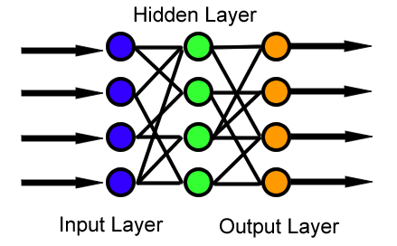
In the feedforward neural network, information is moved from the input layer through a series of non-linear transformations in the hidden layers, and then makes a prediction after passing through the output layer as Figure 1 shows below. When the neural network is making a scalar prediction, then the output layer has a single node.[¹] The input layer represents the features, with each feature being a different node. Assuming there are \(n_x\) features in the input layer, \(n_1\) nodes in the first hidden layer, and a single output node then there would be \(n_x \times n_1\) edges (or weights) going from the input to the first-hidden layer and \(n_1 \times 1\) edges from the hidden layer to the output node. As hidden layers continue to be added it is easy to see how the number of weights will grow quite quickly. There are also additional weights for the intercept terms which will be talked about later.

Figure 1: Feedforward architecture

Cox-model as a neural network

When there is just a single output node and no hidden layers, then the feedforward neural network acts as a generalized linear model corresponding to the associated loss function. Recall from the previous post that when modelling survival data with the proportional hazards regression (or Cox) model, the loss function is as follows for the \(i^{th}\) observation:

Where \(p_i\) and \(p_j\) are the predicted risks for observations \(i\) and \(j\) , \(\delta_i\) is a censoring indicator for patient \(i\), and \(r_j(t_i)\) is an indicator of whether patient \(j\) was alive at time \(i\). The loss function associated with the Cox model is different from most regression models in that an individual’s loss is conditional on its predictions relative to all other observations. In the event of tied survival times some additional adjustments need to be made, but the examples in this post will all have unique event times. The loss function will therefore be:

coxloss <- function(p,i,delta,time) {
  idx <- (time >= time[i])
  loss <- -1*(delta[i]*(p[i] - log(sum(exp(p[idx])))))
  return(loss)
}
print(sprintf('Loss for 3rd observation is: %0.3f',coxloss(p=4:1,i=3,delta=c(0,1,1,1),time=1:4)))

## [1] "Loss for 3rd observation is: 0.313"

Let’s see how the feedforward architecture looks in this case:

Figure 2: NNet as Cox model

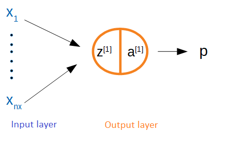
In Figure 2 the output layer is made up of a single node. Define \(z^{[1]}=\sum_{j=1}^{n_x} w_j x_j\) as the linear input to the node and \(a^{[1]}\) as the associated activation function. Since it is also the terminal node it is equivalent to the model’s prediction for that observation: \(a^{[1]}=p\). It is worth pausing to discuss two things: (1) is an intercept needed, and (2) what is the activation function? First, for the output layer of a Cox model no intercept is needed because what matters is the difference in risks rather than their absolute amount, although once there are hidden layers these will have intercepts. Second, in neural networks each node has a corresponding linear input and activation function for two reasons: (i) once there are hidden layers a series of non-linear transformations will be needed because otherwise the system becomes a linear model, and (ii) the output should correspond to a scale that makes sense to the loss function. For example, in binary classification it makes sense to have the output between zero and one to correspond to a probability between the two classes. However in the case of the Cox model, the output activation function can be linear so that \(z=a=p\).

If the dataset (or design matrix) \(\bX=[\bx_1,\dots,\bx_{n_x}]\) in a \(n_x \times m\) matrix then, then for any weight vector \(\bw\) the loss can be evaluated. Note that in the neural network literature, the notation assumes that the columns correspond to the observations and the rows to features. As someone used to thinking as rows as observations, this takes some getting used to. In the code below some fake data is generated.

set.seed(1)
m <- 20
nx <- 2
X <- matrix(rnorm(m*nx),ncol = m)
trueweights <- matrix(c(1,-1),nrow=1)
truerisk <- (trueweights %*% X)
ttrue <- rexp(m,rate=exp(as.vector(truerisk)))
cens <- rexp(m,0.1)
time <- ifelse(cens > ttrue,ttrue,cens)
delta <- as.numeric(cens > ttrue)

Let’s write a function that will loop over all relevant observations to calculate the total loss.

totalcoxloss <- function(w,X,delta,time) {
  event.idx <- which(delta == 1)
  totalloss <- 0
  rskall <- as.vector(w %*% X)
  for (i in event.idx) {
    totalloss <- totalloss + coxloss(rskall,i,delta,time)
  }
  totalloss <- totalloss/length(event.idx)
  return(totalloss)
}
 
w <- matrix(c(1/4,1/4),nrow=1)
 
print(sprintf('Total loss for random weights is: %0.3f',totalcoxloss(w,X,delta,time)))

## [1] "Total loss for random weights is: 2.173"

print(sprintf('Total loss for correct weights is: %0.3f',totalcoxloss(trueweights,X,delta,time)))

## [1] "Total loss for correct weights is: 1.778"

In order to be able to minimize the loss function, the gradient with respect to the weights will need to be found. Since \(p=a=z=\bw \cdot \bx\) in this example, the gradient of the weights can be found by using the information from the \(i^{th}\) sample as follows: \(\frac{\partial \LL_i}{\partial z_i}\frac{\partial z_i}{\partial \bw}\). See this post for more details about the derivation below.

First let’s write a function to find the gradient for the \(i^{th}\) observation at the output layer.

gradcoxoutput <- function(expp,i,delta,time) {
  qset.i <- which(time[i] >= time)
  qvec <- rep(0,length(qset.i))
  for (q in seq_along(qset.i)) {
    qvec[q] <- sum(expp[time >= time[qset.i[q]]])
  }
  grad.i <- -(delta[i]-sum(delta[qset.i]*expp[i]/qvec))
  return(grad.i)
}

Notice that regardless of whether a single observation or all \(m\) observations are used, the gradient with respect to the weights is a \(1 \times n_x\) row vector. When all observations are used, this is referred to as full batch gradient descent, when using a single observation is used stochastic gradient descent (SGD) and when it is some fraction of the observations mini-batch gradient descent. Below is a wrapper that will return the gradients for a given index of observations.

gradcoxbatch <- function(w,X,delta,time,batch) {
  p <- (w %*% X)
  expp <- exp(p)
  gradout <- matrix(0,nrow=1,ncol=length(batch))
  for (i in seq_along(batch)) {
    gradout[,i] <- gradcoxoutput(expp,batch[i],delta,time)
  }
  dw <- (1/length(batch)) * gradout %*% t(X[,batch])
  return(dw)
}
tempgrad <- gradcoxbatch(w,X,delta,time,1:10)
print(sprintf('Gradient directions for full batch w1: %0.2f and w2: %0.2f',tempgrad[1],tempgrad[2]))

## [1] "Gradient directions for full batch w1: -0.14 and w2: 0.85"

Why would one want to use less than all the observations for gradient descent? There are two reasons. First, when the datasets is very large it can be computationally challenging to evaluate all the observations. This is especially true for the Cox model’s gradient which is \(O(m^2)\) to calculate, rather than the usual \(O(m)\) for say linear or logistic regression. Second, when performing gradient descent in high-dimensional space (i.e. many parameters), the initial gradient directions will be “good enough” to get us going in the right direction. An alternative way of phrasing this would be that in many situations many of the \(m\) summands will basically be pointing in the same direction and the information gain of averaging over them will therefore be lessened.

When doing SGD the data needs to randomly sampled every epoch which refers to one cycle through each observation. Lastly the simple gradient descent updating rule can be used until the the loss function approaches an approximate convergence:

Below is one more wrapper to perform SGD.

sgdcoxbatch <- function(w,X,delta,time,alpha,bsize,niter) {
  m <- ncol(X)
  nx <- nrow(X)
  nbatch <- ceiling(m/bsize)
  for (k in 1:niter) {
    set.seed(k)
    batch.idx <- ceiling(sample(1:m)/bsize)
    for (i in 1:nbatch) {
      batch <- which(batch.idx==i)
      dw <- gradcoxbatch(w,X,delta,time,batch)
      w <- w - alpha*dw
    }
    if ((k %% 25)==0) { print(sprintf('epoch %i',k)) } 
  }
  return(w)
}

Let us see how close the model is convergence after 100 epochs with a learning rate of \(\alpha=0.1\) and an initialization of \(\bw = [0,0]\).

library(survival)
mdl.coxph <- coxph(Surv(time,delta) ~ t(X))
what.surv <- coef(mdl.coxph)
 
# Stochastic gradient descent
winit <- matrix(c(0,0),nrow=1)
what.sgd <- sgdcoxbatch(w=winit,X,delta,time,alpha=0.1,bsize=5,niter=100)

## [1] "epoch 25"
## [1] "epoch 50"
## [1] "epoch 75"
## [1] "epoch 100"

round(data.frame(survival=what.surv,sgd=as.vector(what.sgd)),3)

##       survival    sgd
## t(X)1    1.078  1.056
## t(X)2   -0.941 -0.914

The model has basically converged. Note that SGD will never fully converge, because around the global minimum the gradient of each observation will slightly differ. In practice the learning rate is usually set to decay over time so that the model is forced to converge to some point.

L-layer neural networks

This section introduces the framework for thinking about hidden layers in a neural network. As before there is an input layer and a scalar output node, but now there are also \(L-1\) hidden layers. The schema is shown in Figure 3 below. While there are technically \(L+1\) layers of nodes in the diagram, the input layer is considered outside of the count.

Figure 3: L-layer NNet

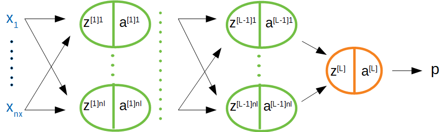
In this following notation: \(z^{[l]k}_{(i)}\) is the linear input corresponding to the \(k^{th}\) node in the \(l^{th}\) layer stemming from the \(i^{th}\) input example, where there are \(n_l\) nodes in the \(l^{th}\) layer. Now as a general rule each linear input will be a function of the previous layer’s activations plus an intercept, which is also referred to as the “bias”. Below the formulas explicitly state the dimensions of each of the terms.

Each layer has it’s own \(n_l \times n_{l-1}\) weight matrix and activation function \(g^{[l]}\). To vectorize across all examples using the entire \(\bX\) matrix the following formulas can be used:

Forward propogation

In order to be able to evaluate the loss function and calculate the hidden activations, a “forward propagation” of the information needs to pass through the neural network. A for-loop will be needed to carry this out since the prediction is necessarily a nested function of \(L\) activations: \(p=a^{[L]}=g^{[L]}(z^{[L]})=g^{[L]}(g^{[L-1]}(z^{[L-1]}))\) and so on. A choice will also need to be made on which activation functions to use in each layer. One of the most popular choices is the rectified linear unit or ReLU function: \(g(x)=x^+=\max [0,x]\). This function is clearly non-linear, but has the nice property that its derivative is very simple: \(g’(x)=x\) if \(x>0\) and \(0\) otherwise.[²] However, ReLU networks can suffer from an unfortunate property known as “ReLU death” when many of the higher level activations are equal to zero. For this reason, the leaky-ReLU function is much more robust: \(g(x)=\gamma x I(x<0) + x I(x>0)\), where \(\gamma\) is a small number (I use 0.1 in the final example).

A function to initialize the weights as well as perform forward propagation is shown below. Because the information across the layers will each have a different dimension, the list object class in R will be appropriate. One list should have named elements corresponding to \(W_1,b_1,\dots,W_L,b_L\) and another, the “cache” with the linear inputs and activations: \(Z_1,A_1,\dots,Z_L,A_L\). For the weight initializer, it is important to make sure the weights do not have too much variance as this can lead to an initial starting point which is stuck in a local minima.

# Weight initialization function
weightinit <- function(layer.dims,nx,ll=1) {
  set.seed(1)
  ldims <- c(nx,layer.dims)
  L <- length(layer.dims)
  weights <- list()
  for (i in seq(length(layer.dims))) {
    namWi <- paste('W',i,sep='')
    nambi <- paste('b',i,sep='')
    weights[[namWi]] <- matrix(runif(ldims[i+1]*ldims[i],-ll,ll),nrow=ldims[i+1])
    weights[[nambi]] <- rep(0,ldims[i+1])
  }
  return(weights)
}
 
# Forward propogation function
forwardprop <- function(weights,X,leaky=0.01) {
  L <- length(weights)/2
  cache <- list()
  for (i in 1:L) {
    namZi <- paste('Z',i,sep='')
    namAi1 <- paste('A',i-1,sep='')
    namAi <- paste('A',i,sep='')
    tempW <- weights[[paste('W',i,sep='')]]
    tempb <- weights[[paste('b',i,sep='')]]
    if (i == 1) {
      tempZ <- (tempW %*% X)
    } else {
      tempZ <- tempW %*% cache[[namAi1]]
    }
    if (i == L) {
      tempA <- tempZ
    } else {
      tempA <- pmax(tempZ,0) + leaky*pmin(tempZ,0)
    }
    cache[[namZi]] <- tempZ
    cache[[namAi]] <- tempA
  }
  return(cache)
}
 
fproploss <- function(cache,delta,time) {
  event.idx <- which(delta == 1)
  totalloss <- 0
  L <- length(cache)/2
  rskall <- as.vector(cache[[paste('A',L,sep='')]])
  for (i in event.idx) {
    totalloss <- totalloss + coxloss(rskall,i,delta,time)
  }
  totalloss <- totalloss/length(event.idx)
  return(totalloss)
}

Let’s compute the loss for a neural network with random weights and layer dimensions of \((3,2,1)\) plus the input layer.

winit <- weightinit(c(3,2,1),2)
cache <- forwardprop(winit,X)
loss <- fproploss(cache,delta,time)
print(sprintf('Loss is %0.3f',loss))

## [1] "Loss is 2.156"

Backward propogation

The most technically challenging part of neural networks is to derive the derivative of each layer’s weights with respect to the loss function. However the task can be approached one layer at a time by calculating three simple partial derivatives with respect to the loss function: (i) the activations, (ii) the linear inputs, and (iii) the weights and the biases. Starting with the terminal layer:

Which is a very similar formulation to the previous case except now the terminal weights are of dimension \(1 \times n_{L-1}\) rather than \(1 \times n_x\) when there was only an output node. Next, consider the penultimate layer.

By iterating back one layer a time, and storing the information in a cache, the derivatives of the weights with respect to the loss function are easy to obtain as the chain rule terms associated with higher level partial derivatives are embedded in just one layer up. The above derivation can be generalized for the \(l^{th}\) layer with some caveats for the output and the input layer. For the leaky-ReLU activation function the derivative will:

# Gradient function for survival-nnet
gradcoxnnet <- function(p,delta,time) {
  haz <- as.vector(exp(p))
  rsk <- rev(cumsum(rev(haz))) 
  P <- outer(haz, rsk, '/')
  P[upper.tri(P)] <- 0
  gradout <- matrix(-1*(delta - (P %*% delta)),nrow=1)
  return(gradout)
}
 
 
# Back propogation function
backprop <- function(weights,cache,X,delta,time,leaky=0.01) {
  L <- length(weights)/2
  m <- sum(delta)
  dcache <- list()
  for (i in seq(L,1,-1)) {
    if (i == L) {
      dA <- gradcoxnnet(p=cache[[paste('A',i,sep='')]],delta,time)
      dZ <- dA
    } else {
      dA <- t(weights[[paste('W',i+1,sep='')]]) %*% dcache[[paste('dZ',i+1,sep='')]]
      dZ <- dA * ifelse(cache[[paste('Z',i,sep='')]]>0,1,leaky)
    }
    if (i == 1) {
      dW <- (1/m) * dZ %*% t(X)
    } else {
      dW <- (1/m) * dZ %*% t(cache[[paste('A',i-1,sep='')]])
    }
    db <- (1/m) * apply(dZ,1,sum)  
    
    dcache[[paste('dZ',i,sep='')]] <- dZ
    dcache[[paste('dW',i,sep='')]] <- dW
    dcache[[paste('db',i,sep='')]] <- db
  }
  return(dcache)
}

Parameter updating

As before the simple gradient descent updating rule can be used to adjust the weights in a direction that will reduce the loss.

# Function to update parameters with the backprop
updateweights <- function(weights,dcache,alpha) {
  L <- length(weights)/2
  for (i in seq(L,1,-1)) {
    weights[[paste('W',i,sep='')]] <- weights[[paste('W',i,sep='')]] - alpha*dcache[[paste('dW',i,sep='')]]
  }
  return(weights)
}

Bringing it all together

All that remains is have a wrapper that will tie together the weightinit, forwardprop, fproploss, backprop, and updateweights functions.

# Function to fit survival-nnet
survnetfit <- function(layer.dims,X,delta,time,alpha,niter=250,verbose=T,ll=1,leaky=0.01) {
  nx <- nrow(X)
  weights <- weightinit(layer.dims,nx,ll)
  
  tord <- order(time)
  time <- time[tord]
  delta <- delta[tord]
  X <- X[,tord]
  
  for (k in 0:niter) {
    cache <- forwardprop(weights,X)
    loss <- fproploss(cache,delta,time)
    dcache <- backprop(weights,cache,X,delta,time)
    weights <- updateweights(weights,dcache,alpha)
    if (((k %% 25)==0) & verbose) { print(sprintf('iter: %i, loss: %0.2f',k,loss))}
  }
  
  return(weights)
}
 
 
# Function to make hazard predictions
survnetpred <- function(snetweights,X,leaky) {
  cache <- forwardprop(snetweights,X,leaky)  
  AL <- as.vector(cache[[length(cache)]])
  return(AL)
}

A simulated example

To show the power of neural networks, the simulated data below will use a non-linear hazard function, specifically: \(h(t;\bx) \propto (x_1^2 + x_2^2)\). The non-linear structure of the neural network will easily be able to learn this quadratic relationship between the features and the associated hazard. There will be a total of 1000 training examples, and 500 test samples will be used to calculate the concordance index. The neural network model will have 3 hidden layers, with (10,5,1) nodes in each layer, respectively.

# Generate the data
m <- 1500
nx <- 2
set.seed(1)
X <- matrix(rnorm(m*nx),ncol=m)
df <- data.frame(t(X))
rsk <- (df$X1^2 + df$X2^2)
tt <- rexp(m,rate=exp(rsk))
cc <- rexp(m,0.25)
delta <- ifelse(cc > tt,1,0)
time <- ifelse(delta==1,tt,cc)
trainX <- X[,1:1000]
testX <- X[,-(1:1000)]
traindf <- df[1:1000,]
testdf <- df[-(1:1000),]
So.train <- Surv(time=time[1:1000],event=delta[1:1000])
So.test <- Surv(time=time[-(1:1000)],event=delta[-(1:1000)])
 
# Cox model
mdl.coxph <- coxph(So.train ~ .,data=data.frame(traindf))
pred.coxph <- predict(mdl.coxph,newdata = data.frame(testdf))
conc.coxph <- survConcordance(So.test ~ pred.coxph)$concordance
 
# Neural network
mdl.snet <- survnetfit(c(10,5,1),trainX,So.train[,2],So.train[,1],alpha = 0.1,niter=250,verbose=F,ll=1/2,leaky=0.1)
 
pred.snet <- survnetpred(mdl.snet,testX,leaky=0.25)
conc.snet <- survConcordance(So.test ~ pred.snet)$concordance
 
print(sprintf('Concordance scores for Cox-PH: %0.3f and neural network: %0.3f',conc.coxph,conc.snet))

## [1] "Concordance scores for Cox-PH: 0.493 and neural network: 0.788"

As the simulation results show, the addition a few hidden layers is able to capture a quadratic hazard relationship without the researcher needing to know the true data generating process. This post has shown how the feedforward neural network architecture can be modified to accommodate survival data by using the Cox partial likelihood loss function at the terminal node. For larger scale projects many additional components need to be incorporated in the neural network model to ensure that the training happens in a reasonable amount of time (by modifying the gradient descent procedure) and does not overfit the data (by adding regularization).

Footnotes