Background and motivation

Before machine learning (ML) algorithms can be deployed in real world settings, an estimate of their generalization error is required. Because data is finite, a model can at most be trained on \(N\) labelled samples \(S=\{(y_1,\bx_1),\dots,(y_N,\bx_N)\}\), where \(y_i\) is the response and \(\bxi\) is a vector of features. Should all \(N\) samples be used in the training of an algorithm? The answer is no for two reasons: (1) hypothesis selection, and (2) generalization accuracy.

First, ML researchers do not limit themselves to a single model, but allow their algorithms to search a space of functions \(\fH=\{h_1,\dots,h_m \}\), for example:

Where \(\Gamma\) is a hyperparameter. A learning algorithm is a map that looks at some number of training samples \(R \subseteq S\) and selects from \(\fH\) a function \(f_R : \bx \to y\), with the goal to minimize some loss function and have \(f_R(\bx) \approx y\).[¹] By learning weights (\(\bbeta\)) indexed by a hyperparameter (\(\Gamma\)) on \(R\), and then seeing how that function performs on a validation set \(V \subseteq S \setminus R\), a fair competition can be had, so that models which overfit on \(R\) are not unduly selected. In other words, by splitting \(S\) into a training set \(R\) and validation set \(V\), we can find for some loss function \(L\):

Second, while the training/validation split provides an unbiased estimate of the relative generalization performance of each indexed function, it does not provide an unbiased estimate of the winning algorithm’s generalization performance. This is because the winning estimator is picked after the data has been observed, so that the error rate is optimistic. For example consider \(m\) i.i.d random normals \(X_i\) with means \(\mu_1 < \mu_2 < \dots \mu_m\), it will be the case that \(E[\min(X_1,\dots,X_m)]<\mu_1\). In other words, if we pick the lowest realization of a vector of normals with different means, our average pick will be lower than the smallest mean: i.e. we will have a biased estimate of \(\arg \min_j E[X_j]\). Instead, if we measure the performance of the winning estimator on some test set: \(T \subseteq S \setminus (R \cup V)\), then an unbiased estimate of the generalization error of the chosen algorithm can be determined.

mu1 <- 0
mu2 <- 1
mu3 <- 2
 
sim <- t(replicate(1000,{
  val <- rnorm(n=3,mean=c(mu1,mu2,mu3),sd=rep(1,1))
  c(val[which.min(val)],which.min(val))
}))

## [1] "Mean of smallest realization: -0.28"

## [1] "Relative frequency of winning r.v.s"

## [1] "76.3%" "19.9%" "3.8%"

Therefore in our classical set up, a dataset of \(N\) samples will be split into \(N_R\), \(N_V\), and \(N_T\), in order to train the models (on \(N_R\)), pick the best performing one (on \(N_V\)) and then get an estimate of its performance for observations it hasn’t observed in its training/selection (using \(N_T\)). Note we will assume that the samples are independently drawn from some common distribution: \((y,\bx) \sim P(\by,\bx)\). Going forward, we’ll aggregate \(N_R+N_V\) and call then \(N_R\), because we’re not interested in model selection.

Now consider this question: how many observations should I put aside in \(N_T\) to give me high confidence that my chosen algorithm will perform well? One way to interpret this is to assume the researcher wants to perform inference around their test set performance. Assuming it is a binary classification problem, recall that the the \((1-\alpha)\)% CI around any test set error can be bounded to \(\pm \epsilon\) using either the binomial proportional confidence interval (BPCI) or Hoeffding’s inequality.

The \(N_T\) under Hoeffding’s is always greater than the BPCI, although the latter is only true for sufficiently large \(N_T\) since \(\frac{1}{\sqrt{N}} (\hat{p}-p_0) \overset{d}{\to} N(0,p_0(1-p_0))\). Hoeffding’s inequality also has the nice property that we don’t need to know the value of \(\hat{p}\) or \(p_0\).

The trade-off

Based on equation \eqref{eq:hoeffding}, a researcher can calculate the number of observations they would need to have a 95% CI to be within \(\pm \epsilon\) of the point estimate obtained on the test set. For example, if \(\epsilon=0.05\), this would imply \(N_T=740\). However, this quantity is for the \((1-\alpha)\)-CI of \(E_{P(y,x)}[L(y,f_R(x))] \pm \epsilon = \text{Err}_{f_R} \pm \epsilon\), where Err is the generalization error. The problem is that the expected loss is itself a function of \(N_R\), so there is now a tradeoff between the level of the error and the uncertainty of that error. In other words we can assume:

This is highly intuitive: the more observations given to the training/validation set, the lower the expected generalization error will be because the model has more observations to learn the underlying structure of the data.

Consider this motivating simulation. A binary outcome is generated by a single binary feature: \(p(y_i=1)=\sigma(\beta_0 + \beta_1x_i)\), where \(\sigma\) is the sigmoid function, \(x_i \sim \text{Bern}(0.5)\), and \(\beta_0=-1\) and \(\beta_1=2\). In the simulation below we will split \(N=100\) from \([N_R,N_T]=[10,90]\) to \([N_T,R_T]=[90,10]\) and calculate the uncertainty around the test set point estimate using the binomial confidence interval.

# True model
pix <- 0.5
b0 <- -1
b1 <- +2
expit <- function(x) { 1/(1+exp(-x))}
dclass <- function(x,tt=0.5) { ifelse(x > tt,1,0) }
nsim <- 500
N <- 100
idx <- seq(N/10,N-N/10,N/10)
bayes.rate <- (1-expit(b0+b1))*pix + (expit(b0)-0)*pix
phat.store <- list()
pse.store <- list()
for (k in 1:nsim) {
  set.seed(k)
  x <- rbinom(N,1,prob=pix)
  py <- expit(b0 + b1*x)
  y <- rbinom(N,1,py)
  dat <- data.frame(y,x)
  kpred <- lapply(idx,function(ii) dclass(predict(glm(y~x,family=binomial,data=dat[1:ii,]),
                                      newdata=dat[-(1:ii),],type='response'))==dat[-(1:ii),]$y )
  phat <- unlist(lapply(kpred,mean))
  pse <- mapply(function(phat,N) sqrt(phat*(1-phat)/N),phat,N-idx )
  phat.store[[k]] <- phat
  pse.store[[k]] <- pse
  print(k)
}
error.hat <- 1-apply(do.call('rbind',phat.store),2,mean)
pse.hat <- apply(do.call('rbind',pse.store),2,mean)
dat.hat <- data.frame(error=error.hat,pse=pse.hat,Ntrain=idx)

Figure: Trade-off between \\(N_R\\) and \\(N_T\\)

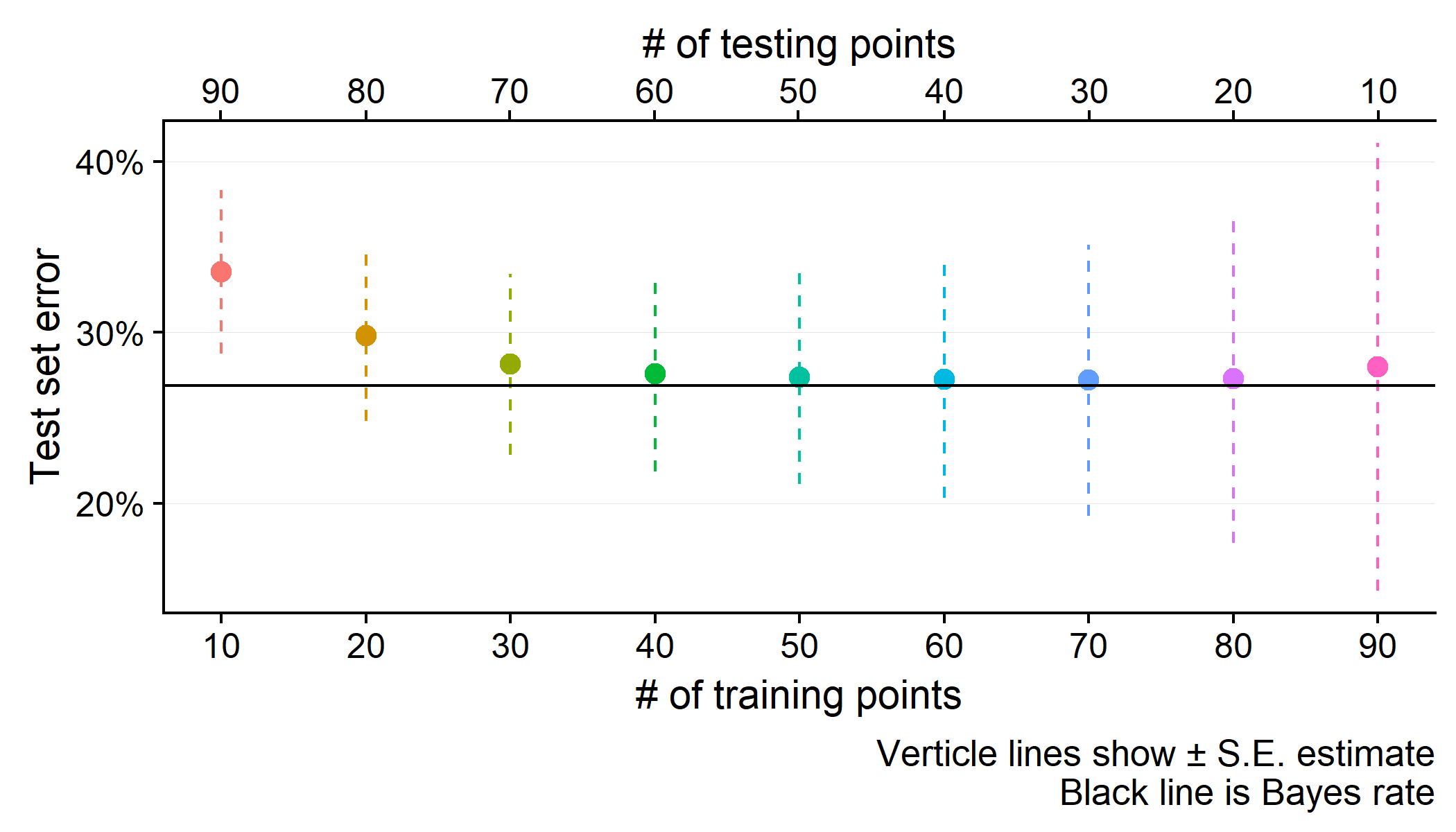
As the Figure above shows, the generalization error continues to fall until round \(N_R=40\), at which point it nearly reaches the Bayes rate (the error obtained if the true parameter values were known). At the same time, at \([N_R,N_T]=[80,20]\) the uncertainty around the test set accuracy has an upperbound close to the level under \([N_R,N_T]=[20,80]\)! In other words, even though this model will generalize close the best possible error rate, we would not be confident in our assessment of its performance.

Summary

This post has shown that there is a trade-off that occurs between the level of the generalization accuracy and the uncertainty around this measurement on the test set. Specifically, as the number of samples committed to the training/validation sets increase, the average generalization error will fall towards the Bayes Rate of the given hypothesis class, while at the same time, the confidence interval around that point estimate will increase.

What the “best” apportionment will be will depend on what the research objectives are. For example, if the goal of our binomial regression model above was to find the model which had the lowest upper bound from the 95% CI, then \([N_R,N_T]=[40,60]\) would be the optimal choice. However, learning these two parameter weights is statistically quite easy, and in more complex settings, the split would likely be more biased towards \(N_R\). In summary there is no simple solution to determining how best to apportion a machine learning dataset to the different training/test/validation sets. It will depend on how efficiently the model learns from data, how stable the model is under different hyperparameter levels, and how much the researcher cares about quantifying test set uncertainty.

Footnotes