This posts outlines the paranet package, which allows for the fitting of elastic net regularized parametric survival models with right-censored time-to-event data in python. I became interested in this topic when I realized that the a parametric modelling excercise would be useful for a business case, but was unable to find any package support in python. Currently, paranet supports three parametric distributions: i) Exponential, ii) Weibull, and iii) Gompertz. These distributions were chosen due to their common usage in practice and for their computational simplicity since sampling and quantile calculations can be done trivially with the inverse method. Adding additional distributions to support non-monotonic hazard rates could a possible future release.

Parametric model support currently exists with the lifelines and pysurvival packages, but these packages do not support regularization for these model classes. Elastic net survival models can be fit with the scikit-survival package, but this is only for the Cox-PH model. While the Cox model is a very important tool for survival modelling, its key limitation for large-scale datasets is that i) it is not natively able to do inference on individual survival times, and ii) its loss function is non-parametric in that its run-time grows O(n^2) rather than O(n).

The paranet package allows users to fit a high-dimensional linear model on right-censored data and then provide individualized or group predictions on time-to-event outcomes. For example, fitting a parametric model on customer churn data can allow a data science to answer interesting questions such as: “out of these 100 customers, when do we first expect that 10% of them will have churned?”, or “for this new customer, at what time point are they at highest risk of leaving us (i.e. maximum hazard)?”, or “for an existing customer, what is the probability they will have churned in 10 months from now?”.

The paranet package is available on PyPi and can be installed with pip install paranet=0.1.4. NOTE this package has been tested with python 3.9+. Using earlier versions of python may lead to errors.

The rest of the this post is structured as follows. Section (1) provides an overview of the basic syntax of the package, section (2) details how the three distributions are parameterized and how covariates effect the scale parameter, section (3) explains how censoring is carried during random variable generation, section (4) gives a high-level overview on high optimization is carried out, and sections (5) to (7) provide code block examples of how to carry out basic model fitting, visualize individualized hazard and survival functions, and do hyperparameter tuning.

(1) Basic syntax

The parametric class is the workhouse model of this package. When initializing the model users will always need to the specify the dist argument. This can be a list or a string of valid distribution types. There are no limits on how long this list can be, but if it is of length k, then subsequent time measurements will either need to a vector or a matrix with k columns.

Although each input argument is defined in the docstrings, several parameters will recur frequently throughout and are defined here for convenience.

1. x: An (n,p) array of covariates. Users can either manually add an intercept and scale the data, or set add_int=True and scale_x=True.
2. t: An (n,k) array of time measurements that should be non-zero. If \(k\geq 0\) then the model assumes each column corresponds to a (potentially) different distribution.
3. d: An (n,k) array of censoring indicators whose values should be either zero or one. As is the usual convention, 0 corresponds to a censored observation and 1 to an un-censored one.
4. gamma: The strength of the regularization (see section (2) for a further description). If this variable is a vector or a matrix, it must correspond to the number of columns of x (including the intercept if it is given).
5. rho: The relative L1/L2 strength, where 0 corresponds to L2-only (i.e. Ridge regression) and 1 corresponds to L1-only (i.e. Lasso).

As a rule paranet will try to broadcast where possible. For example, if the time measurement array is t.shape==(n,k), and dist=='weibull' then it will assume that each column of t is a Weibull distribution. In contrast, if t.shape==(n,) and dist=['weibull','gompertz'], it broadcast copies of t for each distribution.

The parametric class has X keys methods. If x, t, or d are initialized then arguments can be left empty.

1. fit(x, t, d, gamma, rho): Will fit the elastic net model for a given gamma/rho penalty and enable methods like hazard to be executed.
2. find_lambda_max(x, t, d, gamma): Uses the KKT conditions of the sub-gradient to the determine the largest gamma that is needed to zero-out all covariates except the scale and shape parameters.
3. {hazard,survival,pdf}(t, x): Similar to predict is sklearn, these methods provide individualized estimates of the hazard, survival, and density functions.
4. quantile(percentile, x): Provides the quantile of the individualized survival distribution.
5. rvs(n_sim, censoring): Generates a certain number of samples for a censoring target.

When initializing the parametric class, users can include the data matrices which will be saved for later for methods that require them. However, specifying these arguments in later methods will always override (but not replace) these inherited attributes.

1. dist: Required argument that is a string or a list whose elements must be one of: exponential, weibull, or gompertz.
2. alpha: The shape parameter can be manually defined in advance (needs to match the dimensionality of dist).
3. beta: The scale parameter can be defined in advance (needs to match the dimensionality of dist and x).
4. scale_x: Will standardize the covariates to have a mean of zero and a variance of one. This is highly recommended when using any regularization. If this argument is set to True, always provide the raw form of the covariates as they will be scaled during inference.
5. scale_t: Will normalize the time vector be a maximum of one for model fitting which can help with overflow issues. During inference, the output will always be returned to the original scale. However, the coefficients will change as a result of this.

(2) Probability distribution parameterization

Each parametric survival distribution is defined by a scale \(\lambda\) and, except for the Exponential distribution, a shape \(\alpha\) parameter. Each distribution has been parameterized so that a higher value of the scale parameter indicates a higher “risk”. The density functions are shown below. The scale and shape parameters must also be positive, except for the case of the Gompertz distribution where the shape parameter can be positive or negative.

When moving from the univariate to the multivariate distribution, we assume that scale parameter takes is an exponential transform (to ensure positivity) of a linear combination of parameters: \(\eta\). Optimization occurs by balancing the data likelihood with the magnitude of the coefficients, \(R\):

(3) How is censoring calculated?

When calling the parametric.rvs method, the user can specify the censoring value. In paranet, censoring is generated by an exponential distribution taking on a value that is smaller than the actual value. Formally:

There are of course other processes that could generate censoring (such as type-I censoring where all observations are censored at a pre-specified point). The reason an exponential distribution is used in the censoring process is to allow for a (relatively) simple optimization problem of finding a single scale parameter, \(\lambda_C\), which obtains an (asymptotic) censoring probability of \(\phi\):

Where \(F_C(u)\) is the CDF of an exponential distribution with \(\lambda_C\) as the scale parameter, and \(f_T(u)\) is the density of the target distribution (e.g. a Weibull-pdf). Finding the scale parameter amounts to a root-finding problem that can be carried out with scipy. Finding a single scale parameter is more complicated for the multivariate case because an assumption needs to be made about the distribution of \(\lambda_i\) itself, which is random. While it is tempting to generate a censoring-specific distribution (i.e. \(C_i\)) this would break the non-informative censoring assumption since the censoring random variable is now a function of the realized risk scores. The paranet package assumes that the covariates come from a standard normal distribution: \(x_{ij} \sim N(0,1)\) so that \(\eta_i \sim N(0, |\beta|^2_2)\), and \(\lambda_i \sim \text{Lognormal}(0, |\beta|^2_2)\). It is important that the data be at least normalized for this assumption to be credible.

Where \(f_{i}(u)\) is the density of the target distribution evaluated at \(u\), whereas \(f_\lambda(i)\) is the pdf of a log-normal distribution evaluated at \(i\). This is a much more complicated integral to solve and paranet currently uses a brute-force approach at integrating over a grid of values rather than using double quadrature as the latter approach was shown to be prohibitively expensive in terms of run-time.

(4) How does optimization happen?

Unlike glmnet, the paranet packages does not use coordinate descent (CD). Instead, this packages uses a smooth approximation of the L1-norm to allow for direct optimization with scipy as shown below. Parametric survival models are not easily amenable to the iteratively-reweighted least squares (IRLS) approach used by glmnet, because of the presence of the shape parameter. In contract, an exponential model can be easily fit leveraging existing CD-based elastic net solvers. Moving to proximal gradient descent would enable for direct optimization of the L1-norm loss and represents a possible future release.

(5) Basic usage

In this example, data will be simulated from a Weibull distribution and fit without any regularization, where each observation comes from its “own” distribution which is a function of its covariate values (no censoring occurs):

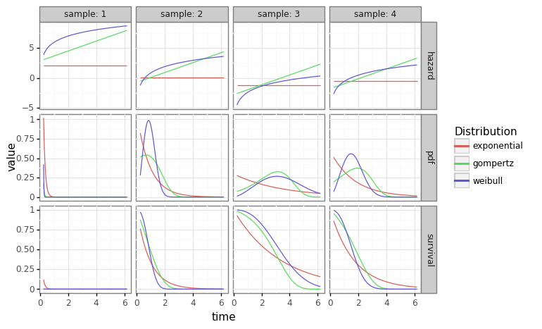
The code block below shows how to fit three parametric distributions to a single array of data generated by covariates. When provided with four “new” rows of data, we can generated individualized hazard, survival, and density curves over the individualized distributions. Notice the exponential distribution (first column) is constant because the exponential distribution’s hazard is constant with respect to time.

# Load modules
import numpy as np
import pandas as pd
import plotnine as pn
from scipy import stats
from paranet.models import parametric

# (i) Create a toy dataset
n, p, seed = 100, 5, 3
x = stats.norm().rvs([n,p],seed)
shape = 2
b0 = 0.25
beta = stats.norm(scale=0.5).rvs([p,1],seed)
eta = x.dot(beta).flatten() + b0
scale = np.exp(eta)
t = (-np.log(stats.uniform().rvs(n,seed))/scale)**(1/shape)
d = np.ones(n)

# (ii) Fit the (unregularized) model
mdl = parametric(dist=['exponential', 'weibull', 'gompertz'], x=x, t=t, d=d, scale_x=False, scale_t=False)
mdl.fit()

# (iii) Plot the individual survival, hazard, and density functions for five "new" observations
n_points = 100
n_new = 4
t_range = np.exp(np.linspace(np.log(0.25), np.log(t.max()), n_points))
x_new = stats.norm().rvs([n_new,p],seed)

# We can then comprehensively calculate this for each method
methods = ['hazard', 'survival', 'pdf']
holder = []
for j in range(n_new):
    x_j = np.tile(x_new[[j]],[n_points,1])
    for method in methods:
        res_j = getattr(mdl, method)(t_range, x_j)
        if method == 'hazard':
            res_j = np.log(res_j)
        res_j = pd.DataFrame(res_j, columns = mdl.dist).assign(time=t_range,method=method, sample=j+1)
        holder.append(res_j)

# Plot the results
res = pd.concat(holder).melt(['sample','time','method'],None,'dist')

gg_res = (pn.ggplot(res, pn.aes(x='time', y='value', color='dist')) + 
    pn.theme_bw() + pn.geom_line() + 
    pn.scale_color_discrete(name='Distribution') + 
    pn.facet_grid('method~sample',scales='free',labeller=pn.labeller(sample=pn.label_both)))
gg_res

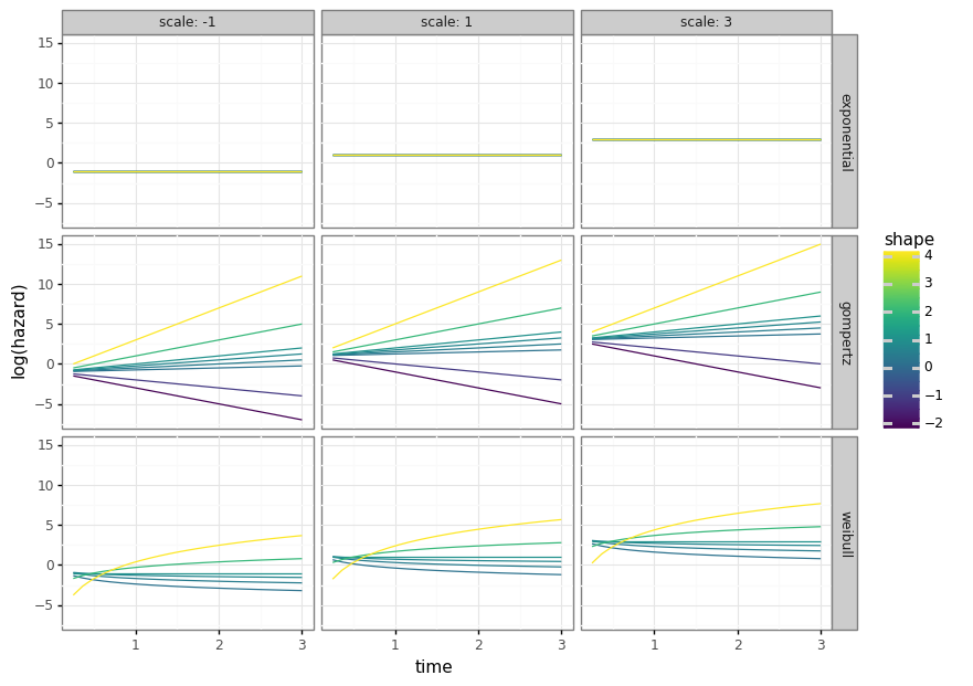
(6) Visualizing shape and scale

The next code block shows how the parametric class can be used to generate the different survival distributions without actually using any data. This is because the model class can be initialized with the alpha (shape) and beta (scale) parameters, which would other otherwise be assigned during the model fitting procedure.

# Example range of shape's for different scales
n_range = 25
t_range = np.linspace(0.25, 3, n_range)
x = np.ones(n_range)
scale_base = np.array([-1, 1, 3])
shape_seq1 = np.array([0.25,0.5,0.75,1,2,4])
shape_seq2 = np.array([-2,-1,0.5,0.5,1,2])
dists = ['exponential', 'weibull', 'gompertz']
holder = []
for scale in scale_base:
    for dist in dists:
        shape_seq = shape_seq1.copy()
        if dist == 'gompertz':
            shape_seq = shape_seq2.copy()
        for shape in shape_seq:
            alpha = np.atleast_2d([shape]*len(dists))
            beta = np.atleast_2d([scale]*len(dists))
            mdl = parametric(dists, alpha=alpha, beta=beta, add_int=False, scale_t=False, scale_x=False)
            df = pd.DataFrame(mdl.hazard(t=t_range, x=x),columns=dists)
            df = df.assign(scale=scale, shape=shape, t=t_range)
            holder.append(df)
res = pd.concat(holder).melt(['t','scale','shape'],var_name='dist',value_name='hazard')

gg_shape_scale = (pn.ggplot(res, pn.aes(x='t',y='np.log(hazard)',color='shape',group='shape')) + 
    pn.theme_bw() + pn.geom_line() + pn.labs(x='time',y='log(hazard)') + 
    pn.facet_grid('dist ~ scale',labeller=pn.labeller(scale=pn.label_both)))
gg_shape_scale

(7) Hyperparameter tuning

This section will show how to tune the \(\gamma\) and \(\rho\) hyperparameters using 10-fold CV so that we are able to fit a model with the best shot of obtaining high performance on a test set. The regularized loss function being minimized for the parametric survival models are:

Where the first term is the (negative) data log-likelihood and the second term is the elastic net penalty. Note that i) there is a tilde over the L1-norm because a smooth convex approximation is used in the actual optimization, and ii) the \(\beta\) (aka scale) parameters ignore index zero which is by tradition treated as an intercept and is therefore not regularized (i.e. \(\beta_0\) and \(\alpha\) are unregularized). Higher values of \(\gamma\) will encourage the L1/L2 norm of the coefficient to be smaller, where the relative weight between these two norms is governed by \(\alpha\). For a given level of \(\gamma\), a higher value of \(\rho\) will (on average) encourage more sparsity (aka coefficients that are exactlty zero).

For a given value of \(\rho>0\), there are a sequence of \(\gamma\) from zero (or close to close) to \(\gamma^{\text{max}}\) that yield the “solution path” of the elastic net model. \(\gamma^{\text{max}}\) is the infimum of gamma’s that achieve 100% sparsity (i.e. all coefficients other than the shape/intercept scale are zero). In practice, it is efficient to start with the highest value of \(\gamma\) and solve is descending order so that we can initialize the optimization routine with an initial value of a less complex model.

The code block below will how to do 10-fold CV to find an “optimal” \(\gamma\)/\(\rho\) combination on the colon dataset using the SurvSet package. To do cross-validation, we split the training data into a futher 10 folds and fit a parametric model on 9 out of 10 of the folds, and make a prediction on the 10th fold and measure performance in terms of Harrell’s C-index (aka concordance). Thus, for every fold, \(\rho\), \(\gamma\), and distribution, there will be an average out-of-fold c-index measure.

The first part of the code loads the data, and prepares an sklearn ColumnTransformer class to impute missing values for the continuous values and do one-hot-encoding for the categorical ones. Because the parametric class (as a default) learns another standard scaler, the design matrix will be mean zero and variance one during training (which is important so as to not bias the selection of certain covariates in the presence of regularization). The SurvSet package is structured so that numeric/categorical columns always have a “num_”/”fac_” prefix which can be singled out with the make_column_selector class. Lastly we do an 80/20 split of training/test data which is stratified by the censoring indicator so that our training/test results are comparable.

# Load additonal modules
from SurvSet.data import SurvLoader
from sklearn.compose import make_column_selector
from sklearn.pipeline import Pipeline
from sklearn.impute import SimpleImputer
from sklearn.compose import ColumnTransformer
from sklearn.preprocessing import OneHotEncoder
from sklearn.model_selection import train_test_split, StratifiedKFold
from sksurv.metrics import concordance_index_censored as concordance
from paranet.models import parametric
from paranet.utils import dist_valid


# (i) Load the colon dataset
loader = SurvLoader()
df, ref = loader.load_dataset('colon').values()
t_raw, d_raw = df['time'].values, df['event'].values
df.drop(columns=['pid','time','event'], inplace=True)

# (ii) Perpeare the encoding class
enc_fac = Pipeline(steps=[('ohe', OneHotEncoder(sparse=False, drop=None, handle_unknown='ignore'))])
sel_fac = make_column_selector(pattern='^fac\\_')
enc_num = Pipeline(steps=[('impute', SimpleImputer(strategy='median'))])
sel_num = make_column_selector(pattern='^num\\_')
enc_df = ColumnTransformer(transformers=[('ohe', enc_fac, sel_fac),('num', enc_num, sel_num)])

# (iii) Split into a training and test set
frac_test, seed = 0.2, 1
t_train, t_test, d_train, d_test, x_train, x_test = train_test_split(t_raw, d_raw, df, test_size=frac_test, random_state=seed, stratify=d_raw)
rho_seq = np.arange(0.2, 1.01, 0.2).round(2)
n_gamma = 50
gamma_frac = 0.001

# (iv) Make "out of fold" predictions
n_folds = 10
skf_train = StratifiedKFold(n_splits=n_folds, random_state=seed, shuffle=True)
holder_paranet, holder_cox = [], []
for i, (train_idx, val_idx) in enumerate(skf_train.split(t_train, d_train)):
    # Split Training data into "fit" and "val" splits
    t_fit, d_fit, x_fit = t_train[train_idx], d_train[train_idx], x_train.iloc[train_idx]
    t_val, d_val, x_val = t_train[val_idx], d_train[val_idx], x_train.iloc[val_idx]
    # Learn data encoding and one-encoded matrices
    enc_fold = enc_df.fit(x_fit)
    mat_fit, mat_val = enc_fold.transform(x_fit), enc_fold.transform(x_val)
    t_hazard_val = np.repeat(np.median(t_fit), mat_val.shape[0])    

    # Fit model
    mdl_para = parametric(dist_valid, mat_fit, t_fit, d_fit, scale_t=True, scale_x=True)
    # Fit along the solution path
    holder_fold = []
    for rho in rho_seq:
        gamma_mat, thresh = mdl_para.find_lambda_max(mat_fit, t_fit, d_fit, rho=rho)
        p = gamma_mat.shape[0]
        gamma_max = gamma_mat.max(0)
        gamma_mat = np.exp(np.linspace(np.log(gamma_max), np.log(gamma_frac*gamma_max), n_gamma-1))        
        gamma_mat = np.vstack([gamma_mat, np.zeros(gamma_mat.shape[1])])
        for j in range(n_gamma):
            gamma_j = np.tile(gamma_mat[[j]], [p,1])
            init_j = np.vstack([mdl_para.alpha, mdl_para.beta])
            mdl_para.fit(mat_fit, t_fit, d_fit, gamma_j, rho, thresh, alpha_beta_init=init_j, grad_tol=0.05)
            # Make out of sample predictions
            res_rho_j = pd.DataFrame(mdl_para.hazard(t_hazard_val,mat_val), columns=dist_valid)
            res_rho_j = res_rho_j.assign(d=d_val, t=t_val, j=j, rho=rho)
            holder_fold.append(res_rho_j)
    # Merge and calculate concordance
    res_rho = pd.concat(holder_fold).melt(['rho','j','t','d'],dist_valid,'dist','hazard')
    res_rho['d'] = res_rho['d'] == 1
    res_rho = res_rho.groupby(['dist','rho','j']).apply(lambda x: concordance(x['d'], x['t'], x['hazard'])[0]).reset_index()
    res_rho = res_rho.rename(columns={0:'conc'}).assign(fold=i)
    holder_paranet.append(res_rho)
# Find the best shrinkage combination
res_cv = pd.concat(holder_paranet).reset_index(drop=True)
res_cv = res_cv.groupby(['dist','rho','j'])['conc'].mean().reset_index()
param_cv = res_cv.query('conc == conc.max()').sort_values('rho',ascending=False).head(1)
dist_star, rho_star, j_star = param_cv[['dist','rho','j']].values.flat
j_star = int(j_star)
idx_dist_star = np.where([dist_star in dist for dist in dist_valid])[0][0]
print(f'Optimal dist={dist_star}, rho={rho}, gamma (index)={j_star}')


# (v) Fit model with the "optimal" parameter
enc_train = enc_df.fit(x_train)    
mat_train, mat_test = enc_df.transform(x_train), enc_df.transform(x_test)
mdl_para = parametric(dist_valid, mat_train, t_train, d_train, scale_t=True, scale_x=True)
# Find the optimal gamma
gamma, thresh = mdl_para.find_lambda_max()
gamma_max = gamma.max(0)
gamma_star = np.exp(np.linspace(np.log(gamma_max), np.log(gamma_frac*gamma_max), n_gamma-1))
gamma_star = np.vstack([gamma_star, np.zeros(gamma_star.shape[1])])
gamma_star = gamma_star[j_star,idx_dist_star]
# Re-fit model
mdl_para.fit(gamma=gamma_star, rho=rho_star, beta_thresh=thresh)

# (vii) Make predictions on test set
t_haz_test = np.repeat(np.median(t_train), len(t_test))
hazhat_para = mdl_para.hazard(t_haz_test, mat_test)[:,idx_dist_star]
conc_para = concordance(d_test==1, t_test, hazhat_para)[0]
print(f'Out of smaple conconcordance: {conc_para*100:.1f}%')

Out of sample concordance: 66.7%

Because each 9/10 fold combination will have a different \(\gamma^{\text{max}}\), we create distribtuion specific sequence (of length 50) down to \(0.001\cdot\gamma^{\text{max}}\) in a log-linear fashion which tends to yield a more linear descrease in the decrease in sparsity. Thus when we when find \(j^{*}\), what we are finding is the index of this sequence. Lastly, we make a prediction on the test set and find that we obtain a c-index score of 66.7%.