Introduction and motivation

In Economics, my previous field of study, empirical research was often interested in estimating the parameters of a theoretical model. Such parameters of interest might include the risk premium embedded in the term structure of interest rates or the elasticity of the labour supply. The main data problem was often finding information at a high enough frequency (in the case of a time series model) or constructing a justifiable proxy. For other fields, data sets can have thousands of features whose theoretical value is ambiguous. In this situation we can appeal to variable reduction methods such as step-wise selection procedures or dimensionality reduction using methods like PCA. Even after this, we may still be left with many plausible variables. At this point using classical linear regresion techniques may be suboptimal due to the risk of overfitting. The problem of overfitting is directly related to the bias-variance tradeoff, in which it may be optimal to have a biased estimator \(f(\theta)\) because the expected mean-squared error may still be lower than an unbiased estimator if the variance is sufficiently reduced:

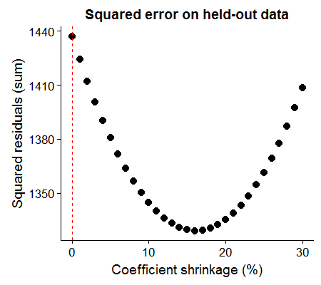
To provide a moviating example, suppose we have \(p=100\) variables and \(n=1000\) observations to model a continuous outcome variable \(y\), and we have to commit to a linear model using only the first 200 observations. Are we better off using the classical regression (OLS) approach, or taking this estimate and shrinking our parameters by 5%? It turns out that the latter approach leads to a lower mean-squared error.

set.seed(1)
n <- 1000
p <- 100
# Generate 1000x100 data set
X <- rnorm(n*p) %>% matrix(ncol=p)
# Create continuous variable as a function of only one feature
beta <- c(2,rep(0,p-1))
y <- (X %*% beta) + rnorm(nrow(X))
# Fit OLS on first 20% of observations
ols <- lm(y~.-1,data=data.frame(y,X)[1:(n/5),]) %>% coefficients %>% matrix
shrink <- ols*0.95
# Test OLS verse shrunken parameters on remaining 80%
X80 <- X[-c(1:(n/5)),]
y80 <- y[-c(1:(n/5))]
ols.error <-  y80 - (X80 %*% ols)
shrink.error <- y80 - (X80 %*% shrink)
# Show error
data.frame(ols.error=ols.error %>% raise_to_power(2) %>% sum,
           shrink.error=shrink.error %>% raise_to_power(2) %>% sum)

##   ols.error shrink.error
## 1  1437.199     1380.593

Using this generated data as an example, we can see that we get the lowest mean squared error on the held-out data when we shrink all of the coefficient parameters by 16%.

At this point it is worth reflecting on two questions: (1) why did we leave out data, and (2) why did we “shrink” the coefficients? To the first point, because we specified the true data generating process (DGP) as \(y = 2X_1 + e\), we wanted to see how poorly the vector of coefficients which minimized the sum of squared residuals on some realization of the data performed as we received more information. This is the advantage of Monte Carlo techniques: we can simulate counterfactuals. To the second, we may want to shrink our parameters when we believe that we are likely incorporating too much noise in our coefficient estimates (and hence lowering the variance of our estimator).

Ridge Regression

This tradeoff between minimizing the sum of squared residuals whilst not “committing” too much to one model realization can be described by the following optimization problem, the solution of which is the Ridge regresssion estimator:

In equation (1) we are minimizing the sum of squared residuals (the first term) and the sum of squared coefficients (the second term), with \(\lambda\) representing our regularization parameter, i.e. the weight we put on our coefficient “budget”. As \(\lambda \to \infty\) we set our coefficients to zero, and \(\lambda=0\) is equivalent to the OLS regression. It turns out that this minimization problem has a closed form solution redolent of the classical form:

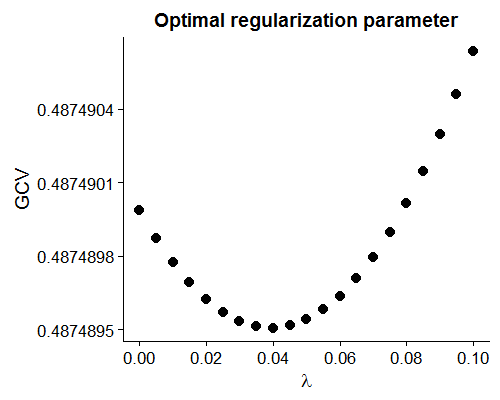
While our motivating example showed that shrinking the coefficients lowered the squared error on the held-out data, how can we decide on a \(\lambda\) term based on the information we have? One common approach is to select a \(\lambda\) which minimizes the Generalized Cross-Validation (GCV) statistic defined as: \(GCV=\frac{1}{n} \sum_{i=1}^n \frac{y_i - \hat{y_i}(\lambda)}{1-tr(\textbf{H})/n}\), where \(\textbf{H}=\bX (\bX’\bX + \lambda I_p)^{-1}\bX’\). Using our simulated data set we see that our GCV recommends a \(\lambda\) of around 0.04.

X20 <- X[1:(n/5),]
y20 <- y[1:(n/5)]
lam <- seq(0,0.1,0.005)
gcv <- rep(NA,length(lam))
for (k in 1:length(lam)) {
  # Calculate H
  H <- X20 %*% solve(t(X20) %*% X20 + lam[k] * diag(rep(1,p))) %*% t(X20)
  # Get fitted value
  y.hat <- t(H) %*% y20
  # And residual
  y.res <- y20 - y.hat
  # Calculate stat
  gcv[k] <- ( (y20 - y.hat)/ (1-diag(H)/nrow(H)) ) %>% raise_to_power(2) %>% mean
}

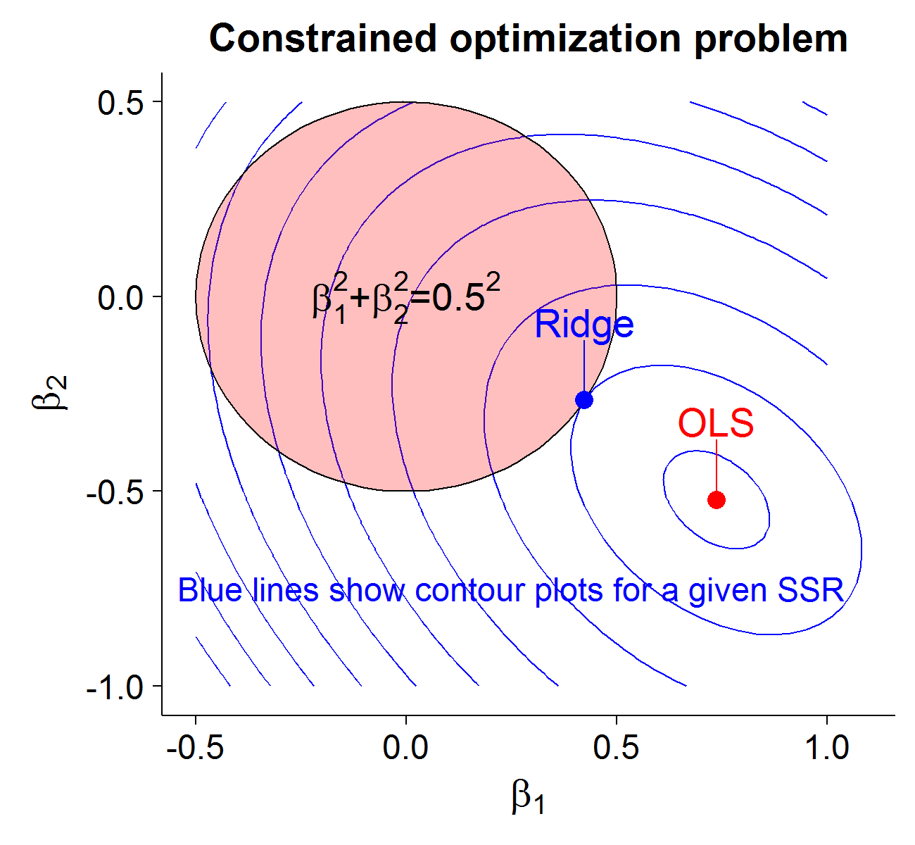
The Ridge regression estimator can also be written as the following constrained optimization problem, i.e. it is equivalent to equations (1) and (2) for some \(\gamma(\lambda)\):

This formulation of the minimization problem is well suited to visualization (for 2-dimensions). We will consider my Craigslist data set gathered over several months for apartment rental prices in Vanouver and Toronto. After normalizing the data (which is required for Ridge regression so that the scale of the variables does not change the results), we model the monthly price as a linear combination of square feet and distance to the downtown core:

Our OLS estimates are \(\hat{\beta_1}\)=0.736 and \(\hat{\beta_2}\)=-0.522. Suppose we set ourselves a “budget” of \(\gamma=0.25\). In equation (3), the first term is equivalent to the sum of squared residuals as a function of \(\beta_1,\beta_2\). It turns out that after we factor our terms, for a given sum of squared residuals \(SSR\) we get the following quadratic curve (i.e. conic section):

Or more generally:

Where \(f= \sum_i price_i^2 - SSR\). This minimization will occur when the contour ellipse intersects with the coefficient budget constraint (which can be represented graphically as a circle: \(\beta_1^2 + \beta_2^2 = 0.25 = 0.5^2\)). The following code generates the Ridge regression estimate and data needed to visualize the constrained optimization solution.

# Function creates points for a circle
circle <- function(r,x0=0,y0=0){
  points <- seq(0,2*pi,length.out=100)
  # Euclidian distance to the origin
  x <- r*cos(points) + x0
  y <- r*sin(points) + y0
  # Return
  return(data.frame(x,y))
}
 
# Constraint circle
gamma <- circle(0.5) %>% tbl_df
 
# Calculate coefficients
attach(norm.dat)
a = sum(ft2^2)
b = 2*sum(ft2*distance)
c = sum(distance^2)
d = -2*sum(ft2*price)
e = -2*sum(distance*price)
f = sum(price^2)
# Create grid
b1 <- seq(-0.5,1,length.out = 100)
b2 <- seq(-1,0.5,length.out = 100)
B <- expand.grid(b1,b2) %>% tbl_df %>% set_colnames(c('b1','b2'))
# And height
B <- B %>% mutate(z=a*b1^2 + b*b1*b2 + c*b2^2 + d*b1 + e*b2 + f)
 
# Find the Ridge coefficients that match constraints
X <- norm.dat[,-1] %>% as.matrix
y <- norm.dat[,1] %>% as.matrix
r <- sum(beta^2)-0.5^2
lam <- 0
# Loop it
while (abs(r) > 0.0001) {
  # Update lambda based on r
  lam <- lam + 100/(1-r)^2*ifelse(r>0,1,-1)
  # Calculate r based on lambda
  r <-  ( (solve(t(X) %*% X + lam*diag(rep(1,2))) %*% t(X) %*% y) %>% raise_to_power(2) %>% sum ) - 0.5^2
}
# Get Ridge coefficients
beta.ridge <- (solve(t(X) %*% X + lam*diag(rep(1,2))) %*% t(X) %*% y) %>% as.numeric
# Get the SSR at the ridge
ssr.ridge <- (y - X %*% matrix(beta.ridge))^2 %>% sum
 
# Define a function that will convert conic parameters to an ellipse
c2e <- function(Par) {
  if ( Par[1]-Par[3] > 10e-10 ) {
    angle <- atan(Par[2]/(Par[1]-Par[3]))/2
  } else {
    angle <- pi/4
  }
  c <- cos(angle)
  s <-  sin(angle)
  Q <- rbind( c(c,s), c(-s,c) )
  M <- rbind( c(Par[1],Par[2]/2) , c(Par[2]/2, Par[3]) )
  D <- Q %*% M %*% t(Q)
  N <- Q %*% matrix(c(Par[4],Par[5]),ncol=1)
  O <- Par[6]
 
  if ( (D[1,1] < 0) & (D[2,2] < 0) ) {
    D = -D;
    N = -N;
    O = -O;
  }
    
  UVcenter = matrix(c(-N[1,1]/2 / D[1,1], -N[2,1]/2 / D[2,2] ),ncol=1)
  free = O - UVcenter[1,1]*UVcenter[1,1]*D[1,1] - UVcenter[2,1]*UVcenter[2,1]*D[2,2];
 
  XYcenter = t(Q) %*% UVcenter
  Axes = matrix(c(sqrt(abs(free/D[1,1])), sqrt(abs(free/D[2,2])) ),ncol=1)
 
  AA = Axes[1]
  Axes[1] = Axes[2]
  Axes[2] = AA
  angle = angle + pi/2
  
  while (angle > pi) {
    angle = angle - pi;
  }
  while (angle < 0) {
    angle = angle + pi
  }
 
  return(c(XYcenter,Axes,angle))
 
}
# Ellipse parameters
ep <- c2e(c(a,b,c,d,e,f-ssr.ridge))
conic.dat <- calculateEllipse(x=ep[1],y=ep[2],a=ep[3],b=ep[4],
                angle=ep[5]*(180/pi),steps=50) %>% tbl_df %>% set_colnames(c('x','y'))