\(\newcommand{\bzi}{\mathbf{z}_i}\) \(\newcommand{\bZi}{\mathbf{Z}_i}\) \(\newcommand{\bmu}{\boldsymbol\mu}\)

Introduction and motivation

This post will consider how to adjust Kaplan-Meier (KM) survival curves, or non-parametric survival curves more generally, for an observational study setting by using inverse probability weights (IPWs). KM curves are frequently employed in survival analysis and clinical studies as they provide a visually intuitive graphic by which to understand the relative survival trajectories of different groups in addition to being able to handle censoring[¹]. In a randomized control trial setting, the comparison of the survival rates between the “treatment” and “control” groups is an unbiased estimate of the comparative survival rates over time, since, on average, the treatment and control groups will have the same distribution of individuals.

In observational studies however, time-to-failure comparisons will be marred by confounding: variables that are both correlated with the outcome of interest (e.g. survival) and the exposure covariate of interest (e.g. different treatment types) will influence the apparent effect of the exposure of interest on the outcome of interest. Confounding can lead to completely spurious relationships (opera attendance and life expectancy) or an exaggerated effect of a variable (education and income)[²]. For a clinical example, consider comparing the survival rates of a treatment mainly given when cancer has progressed to stage IV, in comparison to one that is given to only early stage patients. Clearly, the latter would appear to be “better” for survival, but this just captures the fact that a different distribution of individuals are treated under two regimes. A procedure that adjusts for confounding will therefore need to account for an asymmetric distribution of individuals between exposure levels.

The most well-known method for accounting for confounding effects is multiple linear regression. Assuming that the model is well-specified, the coefficient weights can be interpreted as a causal change in the response from changing a given covariate, holding everything else constant. In survival analysis, the Cox proportional hazards (PH) model is one of the most-utilized approaches to be able to control for multiple covariates. It can also be used to adjust KM survival curves but only conditional at some value for each of the confounders. This prevents the creation of “general” KM survival curves that compare different treatment effects independent of some some specific level for each each of the confounder.

One statistical solution as discussed in Cole and Hernan (2004) is to adjust the Cox PH model by using IPWs so that only a single exposure covariate is included. By conditioning on IPWs, the probability of receiving the treatment a given individual actually received conditional on baseline confounders, the Cox model need only use the fitted values at the different levels of the exposure, and their effect on survival can be generalized outside of specific confounding covariate values[³]. IPWs are used in a variety of statistical procedures, but can broadly be thought of as “upweighting” unlikely observations (such as receiving a drug usually reserved for late-Stage cancer patients if you are Stage I) so that the weighted distribution of features between different exposure levels in an observational study more closely resembles that of a randomized control trial.

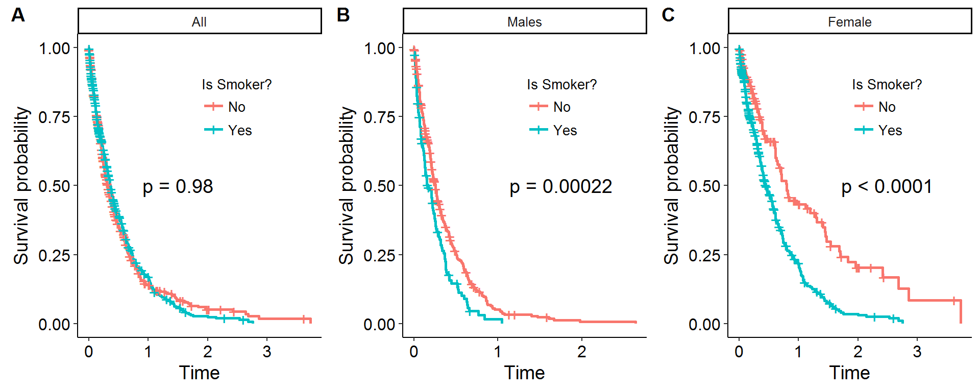
To provide a motivating example with some simulations, consider a theoretical survival curve from an accelerated failure time model: \(S(t;x,z)=S_0(t e^{\beta x + \gamma z})\), where \(x=1\) encodes a smoker, \(z=1\) encodes a male, \(\beta\) and \(\gamma>0\) but \(\text{cor}(x,z) < 0\). In other words, being a smoker and a male “accelerates” the survival path (i.e. one dies faster), but it is assumed that men are less likely to be smokers[⁴]. The values \(\beta,\gamma\) were specifically chosen so that the average survival times between smokers and non-smokers would be comparable. In other words, by having three-quarters of the smokers be female, this toy example provides enough of a confounding relationship to mask the true effect of smoking when seen through the lens of a KM survival curve. Figure 1A displays the result of this confounding, as evidenced by the statistically insignificant log-rank test between the two curves. However, if the KM survival curves are stratified by gender, the true effect of smoking reveals itself, and the log-rank test is able to decisively reject the null of no difference between smokers and non-smokers as Figures 1B and 1C show.

Figure 1: Confounding *in silico*

P-values are for log-rank test

One solution to adjusting KM survival curves is to use stratification at the different levels of the confounders as Figure 1 showed. However, this strategy is undesirable for two reasons: (i) as the number of confounding levels increases from additional covariates the number of observations in each stratified bin will be small making statistical comparisons effectively impossible, and (ii) when confounders are continuous it requires the discritization of the covariates in ways that are not obvious. Therefore, outside of a small number of confounding levels an alternative strategy will be required.

IPWs and Cox PH approach

The statistical solution as proposed by Cole and Hernan (2004) is a three-step procedure:

1. Estimate the IPWs.
2. Estimate a weighted Cox PH model with only one treatment variable.
3. Adjust the KM survival curves with the estimated Cox PH coefficients.

To provide a more formal description of IPWs, consider a sample of \(N\) individuals and for the \(i^{th}\) person denote \(x_i\) as a discrete treatment option (the example below is binary, but it can be multinomial), \(t_i\) and \(\delta_i\) as the observed time and a censoring indicator, \(\bzi\) as a \(p\)-vector of baseline features (possibly confounders), and \(w_i\) as the inverse of the probability of receiving person \(i\)’s treatment \(x_i\) conditional on the observed covariate vector \(\bzi\). The inverse probability weight \(w_i\) can be thought of as the inverse of the conditional marginal density of \(X|Z\): \([f_{X|Z}(x_i|\bzi)]^{-1}\). While \(w_i\) is of course unknown, it can be estimated parametrically, \(\hat{w}_i\), via methods such as logistic regression.

The form that the logistic regression model takes when there is a binary outcome is shown in equation \(\eqref{eq:logit}\). In this generalized linear model, the canonical link is the logit (i.e. log-odds) function, which means a one-unit change in a covariate leads to a \(\mu_j\) unit change in the log-odds of the encoded outcome. As the logit transform is a monotonic transformation of the probability of the event, the conditional probability can always be backed out using the expit transformation[⁵], which allows for the calculation of \(\hat{w}_i\). As \(x_i = {0,1}\)[⁶], one less the fitted probability returns the probability for the alternative event.

\[\begin{align} \log \Bigg( \frac{Pr(X_i=x_i|\bZi=\bzi)}{1-P(X_i=x_i|\bZi=\bzi)} \Bigg) &= \bmu^T\bzi \tag{1}\label{eq:logit} \\ \end{align}\]

Using the fitted coefficients from the logistic regression model, the estimate of the (inverse) of person \(i\) receiving their treatment is shown below.

\[\begin{align*} \hat{w_i} &= [\hat{Pr}(X_i=x_i|\bZi=\bzi)]^{-1} \\ &= \begin{cases} 1+\exp\{-(\hat{\bmu}^T\bzi) \} & \text{ if } x_i=1 \\ 1+\exp\{\hat{\bmu}^T\bzi \} & \text{ if } x_i=0 \\ \end{cases} \end{align*}\]

Recall that IPWs are designed to upweight observations that are “unlikely” within a given treatment group. Thus, if a patient has \(x_i=1\) but the fitted values of the logistic regression are very small, this suggests that this individual is similar in baseline covariates to patients that received \(x_i=0\). Therefore, differences in outcome for this individual are likely to be due to whether they received the treatment and not to some other confounding relationship. However, standard IPWs can suffer from high variance, and the use of stabilized weights is preferred in most settings. As is shown below, this is achieved by normalizing the IPWs by the unconditional probability of treatment. Stabilized weights also have an interesting interpretation when viewed through the lens of stratification. The number of observations in a given confounding strata multiplied by the stabilized weights gives back the “pseudo-population” which is the effective observation weight for that strata.

\[\begin{align*} \hat{sw}_i &= \frac{\hat{Pr}(X_i=x_i)}{\hat{Pr}(X_i=x_i|\bZi=\bzi)} \\ \end{align*}\]

The second step is to estimate a Cox PH model with only a single covariate using IPWs. The standard Cox model is shown in equation \(\eqref{eq:cox}\) below. The hazard rate[⁷] at time \(t\) is described by some baseline hazard function \(h_0(t)\), which is not specified but satisfies the proportional hazards assumption, and a linear combination of features within the natural exponential operator.

\[\begin{align} h(t;\boldsymbol z) &= h_0(t) \exp\{\boldsymbol\gamma^T \boldsymbol z \} \tag{2}\label{eq:cox} \end{align}\]

As is well known in survival analysis, the non-parametric estimate of the survival curve \(\hat{S}(t_j)\) can be estimated through the Kaplan-Meier estimator (or others such as the Nelson-Aalen estimator). Assuming the proportional hazards assumption holds, the coefficients from the Cox regression can be combined with the non-parametric approaches yielding a modified survival curve: \(\hat{S}(t_j) = [\hat{S}_0(t_j)]^{\exp\{\hat{\boldsymbol\gamma}^T \boldsymbol z\}}\). The problem with this approach is that it requires evaluating the \(\boldsymbol\gamma^T \boldsymbol z_0\) term for all values of the \((p+1)\)-vector \(\boldsymbol z\) (assume that \(x_i\) is one of the covariates in the vector).

To solve this problem, the Cox PH regression can be weighted by the IPWs and then estimated with only the single parameter of interest. At a technical level, this is done through the weighting of the partial likelihood of the Cox model as shown below (note that \(R_k(t_i)\) is an indicator function for whether individual \(i\) is alive at time \(t_k\)).

\[\begin{align*} L(\gamma) &= \prod_{i=1}^N \Bigg[ \frac{\exp(\boldsymbol\gamma^T \boldsymbol z)}{\sum_{k=1}^N R_k(t_i) \cdot \exp(\boldsymbol\gamma^T \boldsymbol z) } \Bigg]^{\delta_i} \hspace{3cm} \text{Unweighted partial likelihood} \\ L^{IPW}(\gamma) &= \prod_{i=1}^N \Bigg[ \Bigg( \frac{\exp(\gamma x_i)}{\sum_{k=1}^N R_k(t_i) \cdot \hat{sw}_i \cdot \exp(\gamma x_i) } \Bigg)^{\hat{sw}_i} \Bigg]^{\delta_i} \hspace{1cm} \text{Weighted partial likelihood} \\ \end{align*}\]

Since the weighted-Cox model has only a single covariate \(x_i\), the third and final step is to compare two KM survival curves: \(\hat{S}(t_j;x_i=1) = [\hat{S}_0(t_j;\hat{sw}_i)]^{\exp\{\hat{\gamma}\}}\) and \(\hat{S}(t_j;x_i=0) = \hat{S}_0(t_j;\hat{sw}_i)\).

Example: recurrence of Ewing’s sarcoma

This last section will use the techniques described above with an Ewing’s sarcoma data set referenced in the Cole and Hernan (2004) paper. There are 76 observations on the disease-status of patients that received either a novel treatment (47) or a standard treatment (29), as well as information on whether a patient had abnormally high or normal serum lactic acid dehydrogenase (LDH) enzyme levels. High LDH levels are associated with tumor burden and would be correlated with shorter survival times, ceteris paribus. Figure 2A purports to show that novel treatment improves survival times, and the log-rank test rejects the null of no difference between the two curves at the 5% level. However, Figures 2B and 2C show that after stratifying the survival curves by the two LDH categories, there is no difference in survival times between the novel or standard treatment groups.

Figure 2: Ewing's sarcoma data set

P-values are for log-rank test

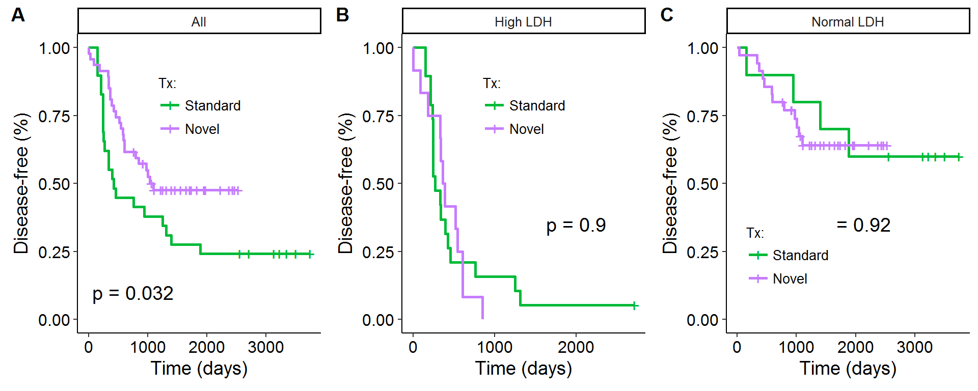
Table 1 below shows the summary statistics for this data set along with information on some of the estimated terms. Notice that while 62% of the patients received the novel treatment, only 39% of the abnormally-high LDH cohort did. Receiving the novel treatment is positively correlated with having better baseline prospects (low LDH), which results in a confounding relationship between survival rates and the treatment. By upweighting high LDH patients with the novel treatment, and normal LDH patients with the standard treatment, the estimate of the survival effect of the treatment will be shown to be insignificant.

Table 1: Stabilized IPWs

LDH	Treatment	N	P(X=x)	P(X=x| Z)	w	sw	Pseudo N
High	Novel	12	0.62	0.39	2.58	1.60	19.20
High	Standard	19	0.38	0.61	1.63	0.62	11.80
Normal	Novel	35	0.62	0.78	1.29	0.80	28
Normal	Standard	10	0.38	0.22	4.50	1.72	17.20

Table 2 shows the estimates of three Cox regression models. In model (1) only the treatment variable is included. For reasons already discussed, this results in a positive bias, and the coefficient estimate suggests that the hazard rate is lower if a patient receives the treatment (significant at the 5% level). However, the inclusion of the LDH variable for model (2) leads to a statistically insignificant measure of treatment variable, and a highly significant one for LDH. Lastly, model (3) shows the coefficient estimate for the different treatments when the model is weighted by the stabilized IPWs. Like model (2), the coefficient result is insignificant, and numerically almost identical[⁸].

Table 2: Cox-PH regression estimates (exponential)

	Biased	Controlled	Weighted
	(1)	(2)	(3)
Treatment	0.53	1.12	1.09
	(0.30, 0.96)	(0.59, 2.11)	(0.60, 1.98)
	p = 0.04	p = 0.74	p = 0.77
LDH status		7.99
		(3.96, 16.13)
		p = 0.00
Observations	76	76	76

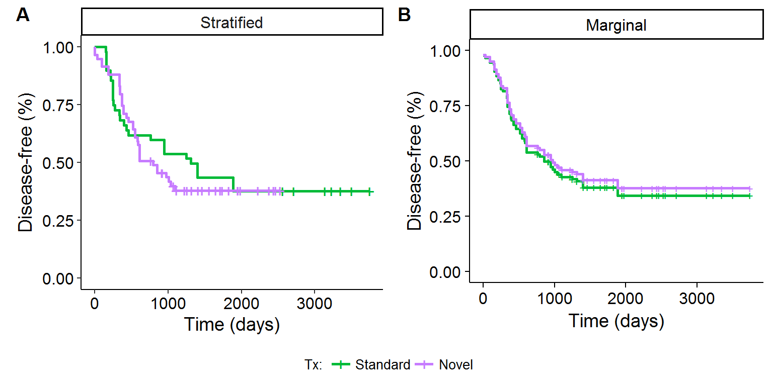
There are actually two approaches that can be used to adjust the KM survival curves: (1) the stratified approach and (2) the marginal approach, as shown in equations \(\eqref{eq:stratified}\) and \(\eqref{eq:marginal}\) below. The former adjusts the estimate of the baseline hazard rate (and hence survival rate[⁹]) for the different treatment levels, whereas the latter shows the theoretical survival distribution for all patients had each person been assigned to the standard or novel treatment. Figures 3A and 3B show the visual results of these two approaches. The stratified approach has the advantage that it uses the same structure of the unadjusted KM curves (and could use the log-rank test in principle), whereas the marginal approach appeals to the potential outcomes framework of the Rubin causal model.

\[\begin{align} \hat{S}_{x}(t_j) &= \hat{S}_{0,x}(t_j) \hspace{2cm} \text{Stratified approach} \tag{3}\label{eq:stratified} \\ \hat{S}(t_j) &= [\hat{S}_0(t_j)]^{\exp\{\hat{\beta} x \}} \hspace{7mm} \text{Marginal approach} \tag{4}\label{eq:marginal} \\ &\text{For } x=\{0,1\} \nonumber \end{align}\]

Figure 3: KM adjusted survival curves

---

References

---

Footnotes

References

Cole, Stephen R., and Miguel A. Hernan. 2004. "Adjusted Survival Curves with Inverse Probability Weights." Computer Methods and Programs in Biomedicine 75: 45-49.
Nieto, Javier, and Josef Coresh. 1996. "Adjusting Survival Curves for Confounders: A Review and a New Method." American Journal of Epidemiology 143: 1059-68.
Robins, J.M. 1998. "Marginal Structural Models." American Statistical Association, Section on Bayesian Statistical Science 1997 Proceedings: 1-10.
Robins, J.M., M.A. Hernan, and B. Brumback. 2000. "Marginal Structural Models and Causal Inference in Epidemiology." Epidemiology 11: 550-60.
Footnotes
-
Censoring occurs when we have information that a patient has survived for at least a certain amount of time, but are unsure of how long they will live for in total. This can be because we haven’t followed up with the individual a second time, or, the study is ongoing so we cannot know the future! ↩
The first confounding relationship is driven purely by lurking variables like income and wealth, whereas the second is inflated because while education does improve your earnings, it is also positively correlated with things like latent ability or personal drive which would also likely increase one’s earnings ↩
To elaborate, without the use of the IPWs, if we wanted to compare two exposure levels taking into account age (a common confounder), there would not be two adjusted KM curves (one for each exposure level), but rather two conditional KM adjusted curves, each of which would be conditioned for a specific age (42, 65, etc). Since the point of a model that uses a linear combination of covariates is to allow for the interpretation of partial effects, this is an undesirable feature of using the standard Cox model. ↩
In the real world, men are actually more likely to be smokers. ↩
\(\log(p/(1-p))=x \longleftrightarrow x=1/(1+e(-x))\) ↩
The zero/one encoding is the conventional notation, but it could \(x_i=\{a,b\}\), as what matters is there are two categorical levels. ↩
Also known as the instantaneous failure rate, the hazard rate can be though of the probability of death at time \(t\) given that one has already survived to \(t\). ↩
IPWs will not for any given estimate produce the same result as a regression model. However, IPWs yield asymptotically unbiased estimators, like multivariate regression, under certain assumptions. ↩
The survival function can be backed out from the cumulative hazard function: \(S(t)=\exp \{- H(t) \}\), where \(H(t) = \int_0^t h(u) du\). ↩