
Building an Elastic-Net Cox Model with Time-Dependent covariates
Introduction
In survival analysis the goal is to model the process by which the rate of events happen. In the applied statistics setting this usually means identifying covariates that are likely to lead to a higher or lower event rate compared to some baseline. When the event is remission or death, a higher event rate corresponds to a riskier patient. One of the unique data challenges in survival modelling is the presence of censoring, which occurs when a patient’s follow-up time is recorded but the event has not yet (or may never) happen.[1] For example, high-risk cancer patients may be monitored for a full year at the end of which some will have passed away and some will still be alive – the latter group having an censored observation at the one-year mark.
The most common model in medical research is the proportional hazards model (which has been discussed in a previous post) which tries to capture the relative order at which patients experience events. In this framework, censored patients can contribute information to modelling the event rate as a censored patient who has lived longer than some patient who experienced the event is likely to be a less risky patient.[2] In many studies with multiple follow-up points a patient’s covariate information changes over time. For example in the heart dataset in the survival package, patient survival is measured while they are on a waiting list for a heart transplant. Below is a snippet of the data.
library(survival)
head(heart)
## start stop event age year surgery transplant id
## 1 0 50 1 -17.155373 0.1232033 0 0 1
## 2 0 6 1 3.835729 0.2546201 0 0 2
## 3 0 1 0 6.297057 0.2655715 0 0 3
## 4 1 16 1 6.297057 0.2655715 0 1 3
## 5 0 36 0 -7.737166 0.4900753 0 0 4
## 6 36 39 1 -7.737166 0.4900753 0 1 4As we can see patient (id) number 3 waited one month before receiving a transplant, and then lived another 15 months before dying. The format of a time-dependent dataset must be put in the long-format as seen above, where every new measurement period is treated as though it were a new observation. This padding additional rows can be thought of as adding left-censored observations (in addition to the standard right-censoring discussed above), as this new “patient” contributes no information to the left of their start time.
While many datasets in survival or time-to-event analysis have these time-dependent properties, there is currently no support for estimating a regularized version of these models using either glmnet or fastcox, the benchmark libraries used for fitting elastic-net models to the proportional hazards loss function. In this post we will show how to build a custom proximal gradient descent algorithm that can incorporate time-dependent covariates.
Elastic-net cox model
To establish the notation, define each observation as having the following tuple: \((t_i^l, t_i^u,\delta_i, \bxi)\), there \(t_i^l\) and \(t_i^u\) are the time periods in which this patient \(i\) had this covariate information, \(\delta_i\) is an indicator of whether the event happened to the patient at \(t_i^u\) and \(\bxi\) is that patient’s vector of covariate measurements. The partial likelihood of the Cox model can be easily accommodated to handle this time-dependent covariate situation.
\[\begin{align} &\text{Partial Likelihood} \nonumber \\ L(\bbeta) &= \prod_{i=1}^N \Bigg( \frac{e^{\bxi^T \bbeta}}{\sum_{j \in R(t_i)}^N e^{\bx_j^T \bbeta}} \Bigg)^{\delta_i} \\ &\text{Partial Log-Likelihood} \nonumber \\ \ell(\bbeta) &= \sum_{i=1}^N \delta_i \Bigg\{ \bxi^T \bbeta - \log \Bigg[\sum_{j\in R(t_i)}^N \exp(\bx_j^T \bbeta) \Bigg] \Bigg\} \tag{1}\label{eq:logpartial} \end{align}\]Where \(\bxi=\bxi(t)\) is now some function of time, and \(R(t_i)\) is the risk-set or index of patients who were alive/non-censored at the event time \(t_i\). Specifically:
\[\begin{align*} R(t_i) &= \{ j \hspace{1mm} : \hspace{1mm} (t_j^u \geq t_i) \wedge (t_j^l < t_i) \} \end{align*}\]The first condition ensures that patient \(j\) either experienced the event or was censored at a later time point than \(t_i\) (and was hence alive when patient \(i\) experienced the event) and the second condition ensures that the start time occurred before the event. Notice that in the heart dataset, the \([t_3^l, t_3^u]=(0,1]\) and \([t_4^l, t_4^u]=(1,16]\) ensuring that patient 3 could never be in his own risk-set twice. It will be useful for downstream computations to use a one-hot encoding matrix of \([\bY]_{ij}=y_i(t_j)\) where \(y_i(t_j)=I[i \in R(t_j)]\).
For high dimensional datasets and prediction problems, the research goal is to find some \(\bbeta\) that balances both model fit (i.e. using all information in the data) as well as maintaining high generalization capabilities (i.e. ignoring dataset-specific noise). Regularization is a technique that returns a coefficient vector which is “smaller” than what would otherwise have been returned, thereby reducing the variance of our model estimate and improving generalization. Furthermore, in high-dimensional settings when there are more features than observations, regularization is also a way to ensure the existence of a unique solution. The elastic-net model combines a weighted L1 and L2 penalty term of the coefficient vector, the former which can lead to sparsity (i.e. coefficients which are strictly zero) and the latter which ensures smooth coefficient shrinkage. The elastic-net optimization is as follows.
\[\begin{align} &\text{Elastic-net loss for the Cox model} \nonumber \\ \bbetah &= \arg \min_{\bbeta} \hspace{2mm} \sum_{i=1}^N \delta_i \Bigg\{ \bxi^T \bbeta - \log \Bigg[\sum_{j\in R(t_i)}^N \exp(\bx_j^T \bbeta) \Bigg] \Bigg\} + \lambda \big( \alpha \| \bbeta\|_1 + 0.5 (1-\alpha) \|\bbeta\|_2 \big) \tag{2}\label{eq:elnet_loss} \end{align}\]The hyperparameter \(\lambda\) in \eqref{eq:elnet_loss} determines the overall level of regularization and \(\alpha\) determines the balance between the sparsest solution possible (\(\alpha=1\) which is the Lasso model) and the zero sparsity approach (\(\alpha=0\) which is the Ridge model). The level of each hyperparameter can be adjusted using methods like cross-validation.
Code base
In the survival package, Surv() objects are used to store the time/event information and can be converted into the \(\bY\) with the following function.
risksets <- function(So) {
  n <- nrow(So)
  Y <- matrix(0,nrow=n, ncol=n)
  if (ncol(So) == 2) {
    endtime <- So[,1]
    event <- So[,2]
    for (i in seq(n)) {
      Y[i,] <- endtime[i] >= endtime
    }
  } else {
    starttime <- So[,1]
    endtime <- So[,2]
    event <- So[,3]
    for (i in seq(n)) {
      Y[i,] <- (endtime[i] >= endtime) & (starttime[i] < endtime)
    }
  }
  return(Y)
}
Here is an example of two different time processes, one that is time-invariant (i.e. start time is always zero) and one that is time-dependent.
So.ti <- Surv(time=c(1,2,3), event=c(0,1,1))
So.td <- Surv(time=c(0,1,0), time2=c(1,10,8), event=c(0,1,1))
risksets(So.ti)
## [,1] [,2] [,3]
## [1,] 1 0 0
## [2,] 1 1 0
## [3,] 1 1 1risksets(So.td)## [,1] [,2] [,3]
## [1,] 1 0 0
## [2,] 0 1 1
## [3,] 1 0 1Because the details of using proximal gradient descent have been outlined in this post I will merely recapitulate the gradient update target we are interested in.
\[\begin{align} &\text{Elastic-net Cox proximal update} \nonumber \\ \bbeta^{(k)} &= S_{\gamma\alpha\lambda}\Bigg(\beta^{(k-1)} + \gamma^{(k)} \Big[ \frac{1}{N}\bX^T(\bdelta - \bP\bdelta) - \lambda(1-\alpha)\bbeta^{(k-1)} \Big] \Bigg) \tag{3}\label{eq:prox_step} \end{align}\]Where \(\gamma^{(k)}\) is the gradient step size at each iteration. Below we outline the code necessary for each component of this update step:
\(S():\)
softhresh <- function(x,t) { sign(x) * pmax(abs(x) - t, 0) }\(\bP\):
Pfun <- function(Y,tY,eta) {
  rsk <- exp(eta)
  haz <- as.vector( tY %*% rsk )
  Pmat <- outer(rsk,haz,'/') * Y
  return(Pmat)
}
\(\bdelta - \bP\bdelta\):
resfun <- function(X, b, Y, tY, l, a, P, d, ll) {
  eta <- as.vector(X %*% b)
  Phat <- P(Y,tY,eta)
  nll <- ll(Phat, d, b, l, a)
  res <- d - Phat %*% d
  return(list(res=res, nll=nll))
}
\(-\frac{1}{N}\bX^T(\bdelta - \bP\bdelta) + \lambda(1-\alpha)\bbeta^{(k-1)}\)
gradfun <- function(X, r, b, l, a) {
  grad <- -t(X) %*% r / nrow(X) + l*(1-a)*b
  return(grad)
}
Equation \eqref{eq:prox_step}:
proxstep <- function(b, g, s, a, l) {
  btilde <- b - s * g
  b2 <- softhresh(btilde, a*l*s)
  return(b2)
}
Equation \eqref{eq:elnet_loss}:
llfun <- function(P,d,b,l,a) {
  -mean(log(diag(P)[d==1])) + l*( a*sum(abs(b)) + (1-a)*sum(b^2)/2 )
}
Lastly, whenever doing convex optimization I prefer to use the Barzilia-Borwien step size adjustment rather than more computational demanding approaches like line search. However for a fully-developed code certain circuit breaks should be included to ensure the step size does not explode in any one iteration.
bbstep <- function(b2, b1, g2, g1) {
  sk <- b2 - b1
  yk <- g2 - g1
  gam <- max(sum(sk*yk)/sum(yk**2),sum(sk**2)/sum(sk*yk))
  return(gam)
}
All of these functions can be combined in a single wrapper elnet.prox.cox shown below.
elnet.prox.cox <- function(So,X,lambda,alpha=1,standardize=T, tol=1e-5,maxstep=1e4, bb=NULL, lammax=F) {
  Y <- risksets(So)
  tY <- t(Y)
  n <- nrow(So)
  p <- ncol(X)
  if (ncol(So)==2) {
    d <- So[,2]
  } else {
    d <- So[,3]
  }

  if (standardize) {
    X <- scale(X)
    mu.X <- attr(X,'scaled:center')
    sd.X <- attr(X,'scaled:scale')
  } else {
    mu.X <- rep(0,p)
    sd.X <- rep(1,p)
  }

  if (is.null(bb)) {
    bhat <- rep(0,p)
  } else {
    bhat <- bb
  }

  # Barzilai Borwein initialization
  res <- resfun(X, bhat, Y, tY, lambda, alpha, Pfun, d, llfun)
  grad <- gradfun(X, res$res, bhat, lambda, alpha)

  gtol <- max(abs(grad))
  if (alpha == 0) { gtol <- gtol / 1e-4 } else { gtol <- gtol / alpha }
  if (lammax) { return(gtol) }
  if (lambda >= gtol) { return(rep(0,p)) }

  bhat.new <- proxstep(bhat, grad, 0.01*gtol, alpha, lambda)
  res.new <- resfun(X, bhat.new, Y, tY, lambda, alpha, Pfun, d, llfun)
  grad.new <- gradfun(X, res.new$res, bhat.new, lambda, alpha)
  gam.new <- bbstep(bhat.new, bhat, grad.new, grad)

  ll.store <- c(res.new$nll,rep(NA,maxstep))
  gam.store <- c(gam.new, rep(NA,maxstep))
  diff <- 1; jj <- 1
  while (diff > tol & jj < maxstep) {
    jj <- jj + 1
    bhat <- bhat.new
    res <- res.new
    grad <- grad.new
    gam <- gam.new

    bhat.new <- proxstep(bhat, grad, gam, alpha, lambda)
    res.new <- resfun(X, bhat.new, Y, tY, lambda, alpha, Pfun, d, llfun)
    grad.new <- gradfun(X, res.new$res, bhat.new, lambda, alpha)
    gam.new <- bbstep(bhat.new, bhat, grad.new, grad)

    ll.store[jj] <- res.new$nll
    gam.store[jj] <- gam.new
    diff <- sqrt(sum((bhat.new - bhat)^2)) / gam
  }

  # re-scale and check KKT
  bhat.scale <- as.vector(bhat / sd.X)

  err.KKT1 <- sum((grad.new[bhat != 0]-alpha*lambda)^2)
  err.KKT2 <- !any(abs(grad.new[bhat == 0]) >= alpha*lambda)
  stopifnot(err.KKT2)

  ll.store <- ll.store[!is.na(ll.store)]
  gam.store <- gam.store[!is.na(gam.store)]
  ret.list <- list(bhat=bhat.scale, err.KKT=err.KKT1, res=as.vector(res.new$res), jj=jj, ll=ll.store, gam=gam.store)

  return(ret.list)
}
Examples
We first want to make sure that elnet.prox.cox can recapitulate the output from coxph in the time-dependent case and glmnet in the time-invariant situation.
library(glmnet)

# Time-invariant data (veteran)
So.ti <- with(veteran,Surv(time,status))
X.ti <- model.matrix(~factor(trt)+karno+diagtime+age+factor(prior), data=veteran)[,-1]

# Time-dependent data (heart)
So.td <- with(heart,Surv(start, stop, event))
X.td <- model.matrix(~age+year+surgery+transplant, data=heart)[,-1]

# (i) Standard cox model
mdl1.coxph <- coxph(So.td ~ X.td,ties = 'breslow')
mdl1.wrapper <- elnet.prox.cox(So.td,X.td,lambda = 0,standardize = T)
round( data.frame(coxph=coef(mdl1.coxph), wrapper=mdl1.wrapper$bhat, row.names = NULL) ,5)
## coxph wrapper
## 1 0.02715 0.02715
## 2 -0.14612 -0.14611
## 3 -0.63584 -0.63584
## 4 -0.01190 -0.01189# (ii) Lasso
l <- 0.05
a <- 1
mdl2.glmnet <- glmnet(X.ti,So.ti,'cox',alpha=a,lambda = l)
mdl2.wrapper <- elnet.prox.cox(So.ti,X.ti,lambda = l, alpha = a)
round( data.frame(glmnet=as.vector(coef(mdl2.glmnet)), wrapper=mdl2.wrapper$bhat ), 5)## glmnet wrapper
## 1 0.04412 0.04419
## 2 -0.02984 -0.02984
## 3 0.00000 0.00000
## 4 0.00000 0.00000
## 5 0.00000 0.00000# (iii) Ridge
l <- 0.1
a <- 0.0
mdl3.glmnet <- glmnet(X.ti,So.ti,'cox',alpha=a,lambda = l)
mdl3.wrapper <- elnet.prox.cox(So.ti,X.ti,lambda = l, alpha = a)
round( data.frame(glmnet=as.vector(coef(mdl3.glmnet)), wrapper=mdl3.wrapper$bhat ), 5)## glmnet wrapper
## 1 0.14798 0.14835
## 2 -0.02931 -0.02930
## 3 0.00247 0.00249
## 4 -0.00170 -0.00170
## 5 -0.09003 -0.09039# (iv) Elastic-net
l <- 0.05
a <- 0.5
mdl4.glmnet <- glmnet(X.ti,So.ti,'cox',alpha=a,lambda = l)
mdl4.wrapper <- elnet.prox.cox(So.ti,X.ti,lambda = l, alpha = a)
round( data.frame(glmnet=as.vector(coef(mdl4.glmnet)), wrapper=mdl4.wrapper$bhat ), 5)## glmnet wrapper
## 1 0.10155 0.10182
## 2 -0.03069 -0.03069
## 3 0.00000 0.00000
## 4 0.00000 0.00000
## 5 -0.00326 -0.00332Of course the point of writing the elnet.prox.cox function is not simply to replicate coxph or glmnet but rather apply it to a regularized time-dependent Cox models. In the code below we will fit the elastic-net solution path for \(\alpha = [1/3, 2/3, 1]\) on the cgd dataset.
head(cgd)## id center random treat sex age height weight
## 1 1 Scripps Institute 1989-06-07 rIFN-g female 12 147 62.0
## 2 1 Scripps Institute 1989-06-07 rIFN-g female 12 147 62.0
## 3 1 Scripps Institute 1989-06-07 rIFN-g female 12 147 62.0
## 4 2 Scripps Institute 1989-06-07 placebo male 15 159 47.5
## 5 2 Scripps Institute 1989-06-07 placebo male 15 159 47.5
## 6 2 Scripps Institute 1989-06-07 placebo male 15 159 47.5
## inherit steroids propylac hos.cat tstart enum tstop status
## 1 autosomal 0 0 US:other 0 1 219 1
## 2 autosomal 0 0 US:other 219 2 373 1
## 3 autosomal 0 0 US:other 373 3 414 0
## 4 autosomal 0 1 US:other 0 1 8 1
## 5 autosomal 0 1 US:other 8 2 26 1
## 6 autosomal 0 1 US:other 26 3 152 1library(cowplot)
library(data.table)
library(forcats)
So.cgd <- with(cgd, Surv(tstart, tstop, status==1))
X.cgd <- model.matrix(~treat+sex+age+height+weight+inherit+steroids+propylac+hos.cat,data=cgd)[,-1]
alpha.seq <- c(1/3, 2/3, 3/3)
bhat.store <- list()
for (alpha in alpha.seq) {
lammax <- elnet.prox.cox(So.cgd, X.cgd, lambda=1, alpha=alpha, lammax=T) # lambda that obtains all zeros
lam.seq <- exp(seq(log(0.01*lammax), log(0.99*lammax), length.out = 100))
bhat.seq <- data.table(lambda=lam.seq, alpha=alpha,
t(sapply(lam.seq,function(lam) elnet.prox.cox(So.cgd, X.cgd, lambda=lam, alpha=alpha)$bhat )))
colnames(bhat.seq)[-(1:2)] <- colnames(X.cgd)
bhat.seq <- melt(bhat.seq,id.vars=c('lambda','alpha'),variable.name='feature')
bhat.store[[as.character(alpha)]] <- bhat.seq
}
bhat.df <- rbindlist(bhat.store)
bhat.df <- merge(bhat.df,bhat.df[,list(l1=abs(sum(value))),by=list(lambda,alpha)],by=c('lambda','alpha'))
bhat.df <- merge(bhat.df,bhat.df[,list(l1max=max(l1)),by=list(alpha)],by='alpha')[order(alpha,feature,lambda)]
bhat.df[, `:=` (a2=alpha, ratio=l1/l1max,
alpha=paste0('alpha==',factor(alpha, levels=names(bhat.store),labels=c('1/3','2/3','1'))))]
bhat.df[, alpha := lvls_reorder(alpha, c(2,3,1))]
gg.solution <-
ggplot(bhat.df, aes(x=log(a2*lambda), y= value,color=feature, group=feature)) +
geom_point() +
facet_wrap(~alpha,labeller = label_parsed, scales='free_x') +
background_grid(major='xy',minor='none') +
labs(x=expression(log(alpha*lambda)),y=expression(hat(beta[j]))) +
ggtitle('Elastic-net solution path') +
theme(legend.position = 'bottom', legend.justification = 'center') +
scale_color_discrete(name='Feature: ')
gg.solution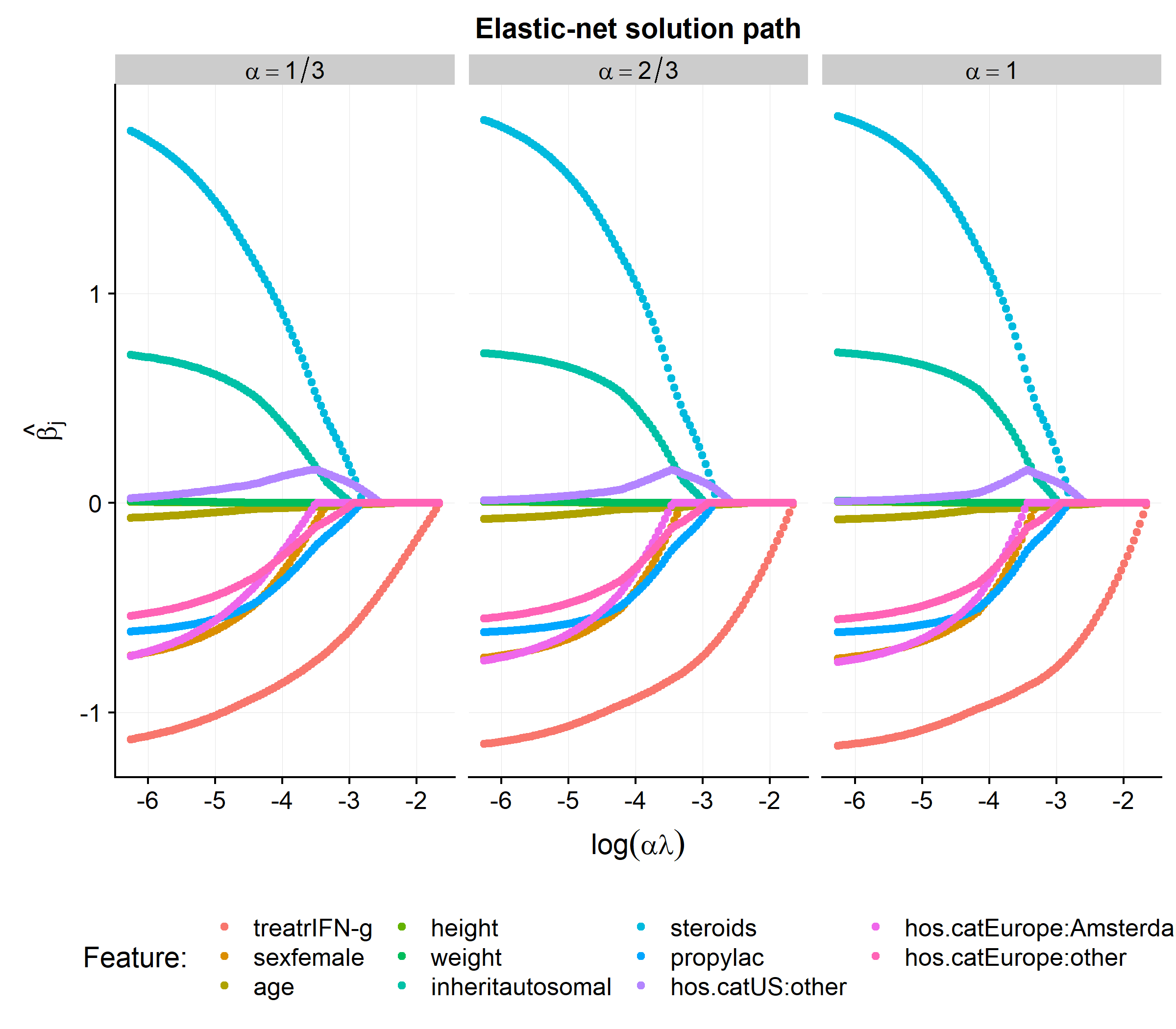
This post has shown how to make minor adjustments to first-order gradient methods to solve the elastic-net Cox model that can handle time-dependent covariate information. In future posts we will explore further algorithmic approaches for estimating a proportional hazard model.
Footnotes
-
The latter scenario technically corresponds to a cure model framework. ↩
-
I say “likely” to be less risky as there is always stochasticity around any process, so that even patients with the same risk profile will realize the event at different times due to the nature of a random processes. Also note that patient who is censored before another patient experiences the event can contribute no information to that pairwise ordering. ↩