Executive summary

A recently published paper in JAMA Network Open by Lee et. al (2021) (hereafter Lee) uses an econometric method which claims to find a deleterious association between the adoption of harm reduction policies at the state level and overdose deaths.[¹] Their method estimates that both Naloxone and Good Samaritan laws increase overdose deaths for up to 12 quarters after policy adoption. I provide three critiques of their analysis with regards to Naloxone and Good Samaritan laws and their relation to overdose deaths.

1. The test statistic does not have a proper distribution under a null hypothesis of no effect. When policy dates are randomized, the Lee method would conclude that Naloxone and Good Samaritan laws increases overdose deaths 35% and 23% of the time, respectively (when it should be 5%).
2. The matching procedure is failing to provide control states which look “similar” to the treated states in terms of overdose deaths. Specifically, the rate of overdose deaths before policy adoption is growing faster in the treated states, which violates the parallel trends assumption needed for inference.
3. The covariates used to generate the propensity score probabilities have a weak relationship to policy adoption.

Since the date of policy adoption determines the coefficient used to assess whether these laws increase overdose deaths, the Naloxone and Good Samaritan results are unreliable since a completely random policy adoption date also leads to a disproportionate number of inferences which suggest the same results. The statistical reason for the inflated type-I error rate is because the standard errors are too small (the null distribution is not a standard normal), and in the case of Naloxone laws there is a non-zero mean. Previous research has suggested similar statistical vulnerabilities: a 2004 QJE paper by Bertrand et. al showed that randomizing policy dates leads to inflated type-I error rates for another type of difference-in-difference estimator.

I also found the matching methods unreliable since the covariates used to generate the propensity scores have a weak relationship to the date of policy adoption. This means that propensity scores used to find matches are noisy. These poor matches in turn lead to a violation of the parallel trends assumption as the gap in opioid deaths between the treatment and control states is growing before as well as after policy adoption. Since the average treatment effect coefficient used in Lee relies on this assumption, the results are confounded.

(1) Background

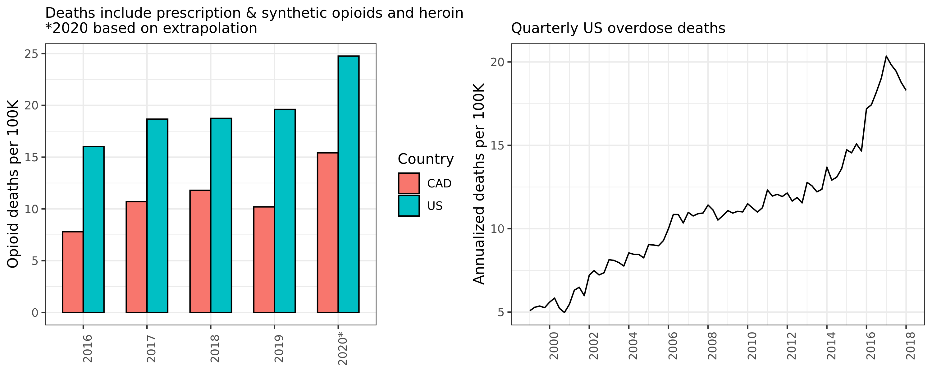
The United States and Canada are experiencing an opioid crisis. The origins of this public health emergency are complex, but “innovations” in prescription opioids (OxyContin and Vicodin), the emergence of new street drugs like black tar heroin and fentanyl, as well as drug criminalization have been posited as primary causes. The annual numbers of opioid overdose deaths in North America are now staggering (see Figure 1).[²] To put these numbers into perspective, the number of fatal motor vehicle crashes and firearms suicides combined (mortality rates of 11 and 8 per 100K persons, respectively) are roughly equivalent to opioid overdose deaths in the US.[³] Although Canada has around half the number of per capita overdose fatalities compared to our southern neighbour, the death rate is still double that of motor vehicle accidents in our country.

Figure 1: US and CAD opioid and overdose deaths

Harm reduction is a public health approach to drug use which stresses the need to reduce the risk of using drugs rather than reducing demand through criminalization or social stigma. “Safe sex”, “drink responsibly”, and seatbelts, are examples of harm reduction approaches to other public health challenges. Recent research by Lee et. al (2021) has called into question the efficacy of harm reduction policies in response to the opioid crisis. This study uses econometric analysis which claims that Naloxone and Good Samaritan policies increase overdose deaths in the long run. The authors use a matching method designed to estimate causal effects of an outcome from a policy adoption in time-series cross-sectional data. This method gives positive coefficient estimates for total overdose deaths up to 12 quarters after policy adoption. The paper defines these harm reduction policies as follows:

1. Good Samaritan laws provide immunity or other legal protection for those who call for help during overdose events.
2. Naloxone access laws provide civil or criminal immunity to licensed health care clinicians or lay responders for administration of opioid antagonists, such as naloxone hydrochloride, to reverse overdose.

What explanation could be given for finding these deleterious effects? The authors do not speculate too much, but they do cite other research that suggests moral hazard may be at work.[⁴]

It is possible that the prospect of getting access to overdose-reversing treatment may instead induce moral hazards by encouraging people to use opioids and other drugs in riskier ways than they would have without the safety net of Naloxone.

…

These unintended consequences may occur if the fundamental causes of demand for opioids are not addressed and if the ability to reverse overdose is expanded without increasing treatment of opioid overdose.

I was sceptical of these findings for two reasons. First, moral hazard only makes sense for explaining an increase of non-fatal opioid overdoses. By definition, in order for naloxone to be a moral hazard, it has to reduce the risk of dying from opioids. It would be strange that something which induces more use because of increased personal safety also killed more people. Second, having worked first an economist and then as an applied statistician for almost an decade, I knew that econometric estimates are sensitive to minor changes in the analysis pipeline. I was curious whether these estimates would be robust to permutation testing and an in-depth analysis.

Lee uses a panel matching method implemented through the PanelMatch package in R. Formally, the method is trying to estimate the difference in the change of the outcomes for up to $F$ periods ahead conditioning on $L$-lags of of the control covariates:

\[\begin{align} &\text{ATT estimator} \\ \delta(F,L) = \frac{1}{\sum_{i=1}^N \sum_{t=L+1}^{T-F} D_{it}} &\Bigg\{ (Y_{i,t+F} - Y_{i,t-1}) - \sum_{i'\in M_{it}} w_{it}^{i'} (Y_{i',t+F} - Y_{i',t-1}) \Bigg\} \tag{1}\label{eq:att} , \end{align}\]

Where \(D_{it}\) is an indicator of whether state \(i\) changed its policy at time \(t\), \(M_{it}\) is the set of control states, \(Y_{it}\) is the outcome, and \(w_{it}\) is the weight for the control state. At every time point, the sum of control weights for a given treated state must be one. This average treatment among the treated (ATT) estimator \eqref{eq:att} is sensitive to the parallel trends assumption since it compares the difference in the difference of levels between the treated and control states (hence it is a type of difference-in-difference estimator).

In the rest of this post I will provide evidence that the econometric results for Naloxone and Good Samaritan laws from Lee are flawed. Though I think this paper needs revisions to address these problems, I applaud the authors for providing reproducible code and data. I also welcome a critique of any of my claims.

(2) Data overview

The authors do an excellent job at making their code and data accessible for researchers. Though the data sources are confidential, Lee provides aggregated measures that can be used in the downstream analysis. This paper should serve as a model for how data-driven social science research is conducted. My analysis in turn was based on code that can be found here.[⁵] The data for the paper comes from several sources including the Optum Clinformatics Data Mart Database, NCHS Multiple Cause of Death file, and Centers for Disease Control and Prevention’s CDC Wonder database.

I focused exclusively on two policy treatments (Naloxone and Good Samaritan laws) and one outcome (total overdose deaths). Though the paper looked at multiple policies and outcomes, I chose to focus on the two harm reduction policies and overdose deaths as I felt these were the most consequential for informing the harm reduction community. Figure 2A shows the underlying dynamics in the different types of overdose deaths in the US. Most opioid categories have seen sky-rocketing deaths (particularly synthetics like fentanyl), and overall opioid deaths have risen measurably to a high level.

Figure 2A: US Opioid deaths over time by category

Figure 2B below shows the cumulative percentage of US states that adopted a harm reduction or supply-controlling policy. By the end of the time series, all states (and DC) had adopted Naloxone laws, and 90% had adopted Good Samaritan laws. A statistical finding that these laws increase deaths is therefore all the more surprising as it implies that all states, eventually, made a policy mistake.

Figure 2B: Cumulative state policy adoption

As mentioned before, Lee’s analysis looked at a variety of policies and outcomes. I calculated the average outcome difference (deaths per 100K) between states which adopted the policy and those that did not (Figure 2C). Confidence intervals where calculated using the quantiles of the difference in bootstrapped means. The dynamics are different between outcomes for the same policy, and policies for the same outcome. Interestingly, there does not appear to be a statistical difference for all overdose deaths for Naloxone laws until after 2016. Of course these are just summary statistics and not counterfactual claims, but it is surprising that there is not a difference between the states given that states with the highest death rates would presumably adopt the laws first.

Figure 2C: Difference on overdose deaths between adopted versus un-adopted states

(3) Failure of the parallel trends assumption

After doing some exploratory analysis, it was clear that the growth rates in overdose deaths between the treated and control states were not equal. Figure 3Ai below shows that the average quarterly percentage change in the overdose deaths before (after) policy adoption in the treated states is 3.1% (2.4%) and 3.4% (2.0%) for Good Samaritan and Naloxone laws, respectively, while their respective control states are 1.4% (1.4%) and 1.6% (1.3%). In other words, the growth rate difference actually falls, on average, after policy adoption! However, because the ATT estimator from \eqref{eq:att} only looks at the difference in levels over time, a deceleration in growth rates can still be recorded as a positive coefficient because the rates are lower in the control group. If anything this evidence points in the opposite direction to the overdose finding from Lee. Figure 3Aii shows that the difference in mean growth rates are statistically different (using a bootstrap quantile method).

A gap in the growth rates of the outcome before policy adoption will almost certainly lead to a violation of the parallel trends assumption. Figure 3Aiii shows this can be visually seen for the Naloxone law case. Although this method of plotting is not completely correct because what matters is the difference in growth between treated and control for each treated state (i.e. multiple growth lines), rather than the growth in the average of levels, the figure clearly shows that even the average of levels still shows a gap in the growth rates before policy adoption.

Figure 3A: Overdose death growth rates between control groups

(i) Observed distribution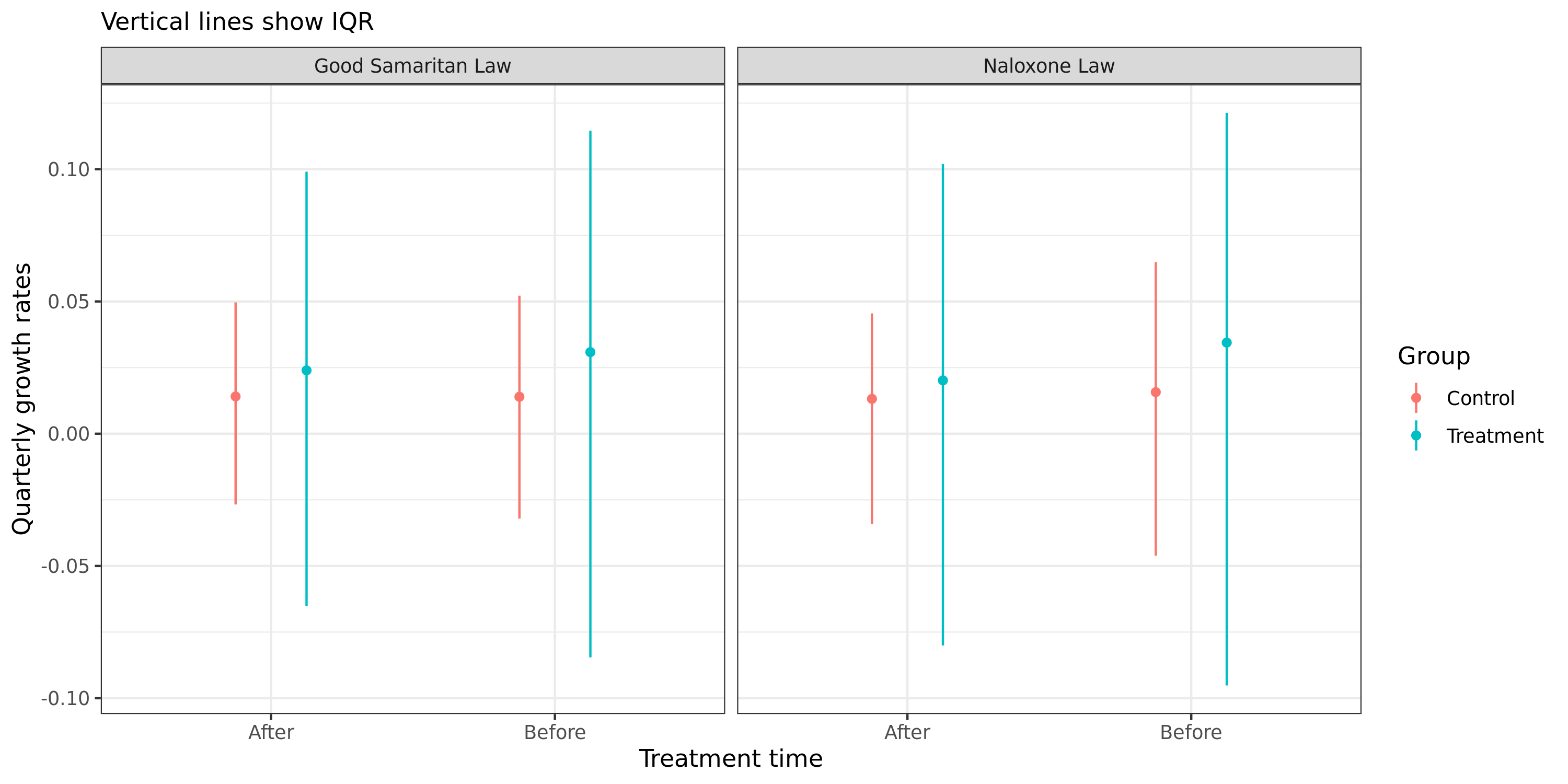

(ii) Bootstrapped difference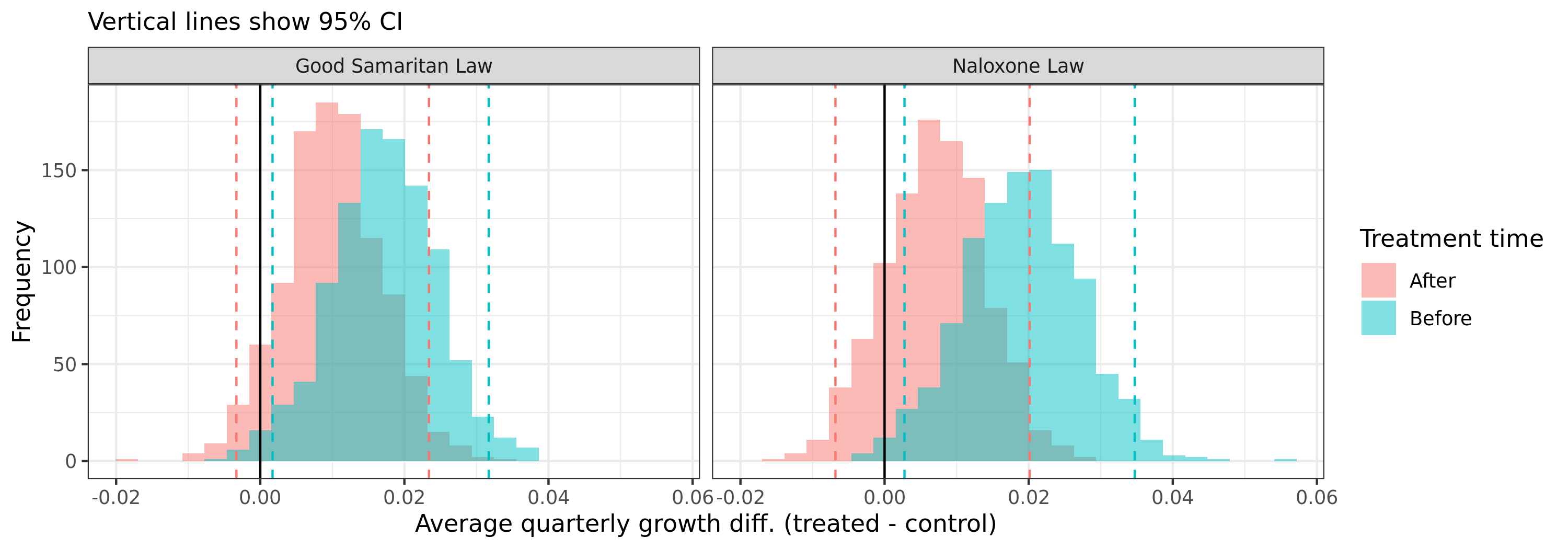

(iii) Violation of parallel trends assumption for Naloxone laws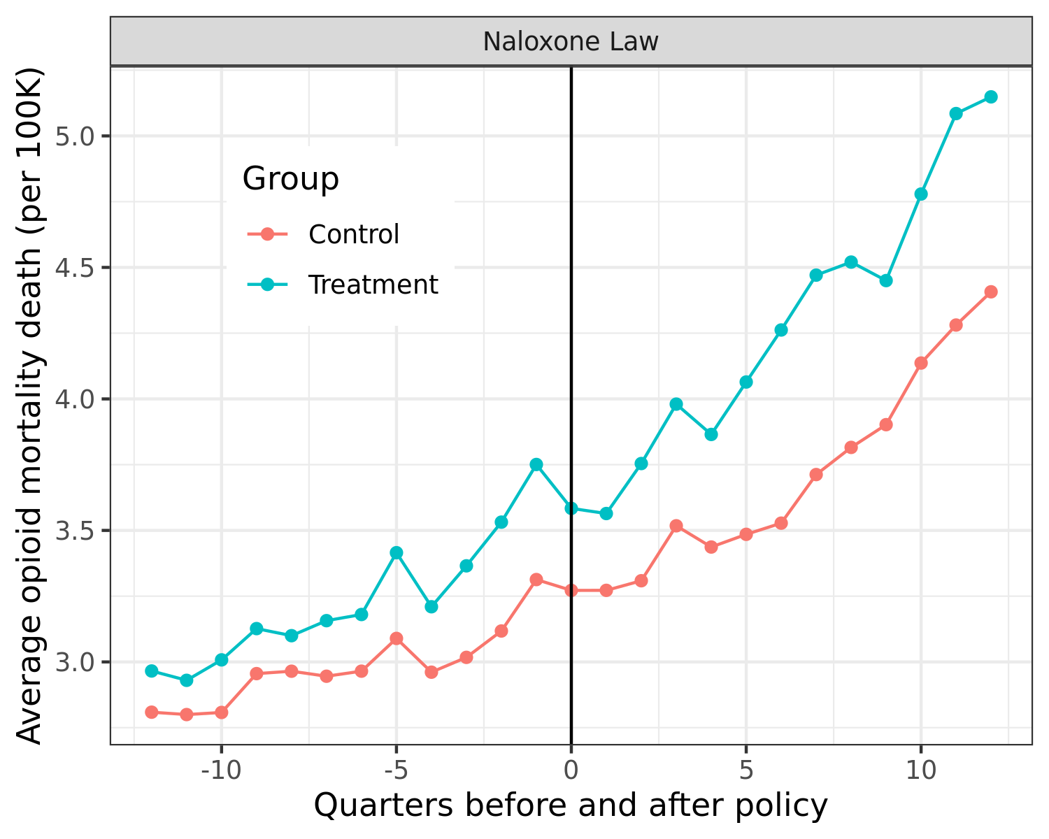

(4) Matching and propensity scores

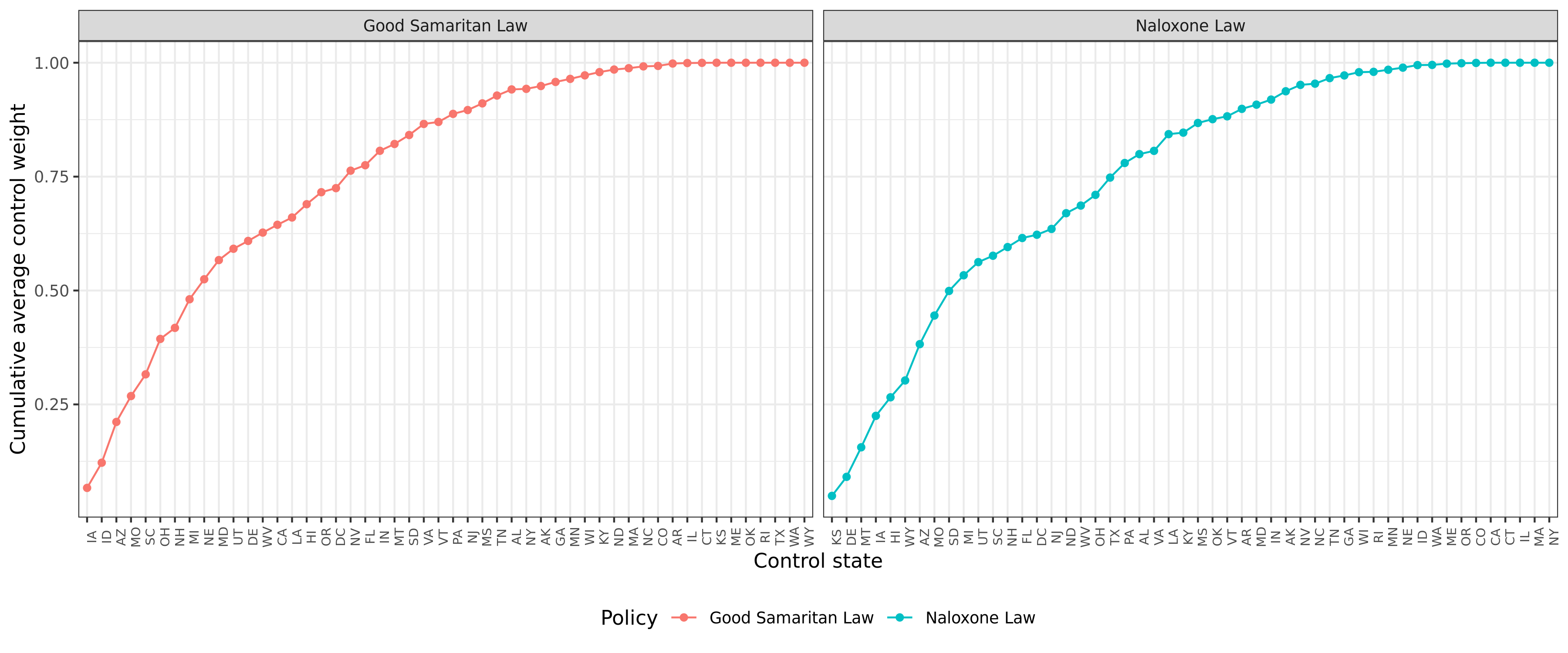
I did not spend too much time analysing the matching method but I did find several results which suggest that the propensity scores are noisy. First, eight states make up 50% or more of the total control weights (Figure 4A). This isn’t problematic per se, but it suggests that removing one or two of these states is likely to influence the subsequent results.

Figure 4A: Control state weights

I also used a logistic regression formulation with the first lag of the control covariates as well as the 12 lags of the outcome data. I found poor predictive performance in terms of the AUROC for predicting the date of policy adoption (see Figure 4B). This result is not definitive as alternative specifications may achieve a better leave-one-state-out AUROC. I could not find any results in Lee that analysed how well the model which generated the propensity scores actually performed when predicting policy adoption.

Figure 4B: Control state weights

(5) Randomizing policy adoption dates

The problems of parallel trends and propensity scores are minor (and possibly fixable) compared to the issue of an inflated and biased test-statistic. As mentioned before, previous econometric work has shown that difference-in-difference estimators do not show the expected null distribution when policy dates are randomized. When the policy date is random, the ATT estimator should have a standard normal distribution. Instead, Figure 5Ai shows that the random-effects meta-analysis (REMA) model has a distribution that is both too wide, and (in the case of Naloxone laws) biased. The z-score estimates found in Lee for the REMA estimate are well within the true null distribution.

Rather strangely, the REMA standard errors tend to be smaller when the coefficient is larger than zero, which causes the z-score to have a right-ward bias, especially in the case of Naloxone laws (Figure 5Aii). Because the z-scores under the null are biased and/or have too high of a variance, the null of no effect would be rejected 35% and 23% of the time in favour of a deleterious relationship between Naloxone and Good Samaritan laws and overdose deaths.

Figure 5A: Z-score and standard error estimates from randomization of policy dates (REMA)

(i) REMA z-score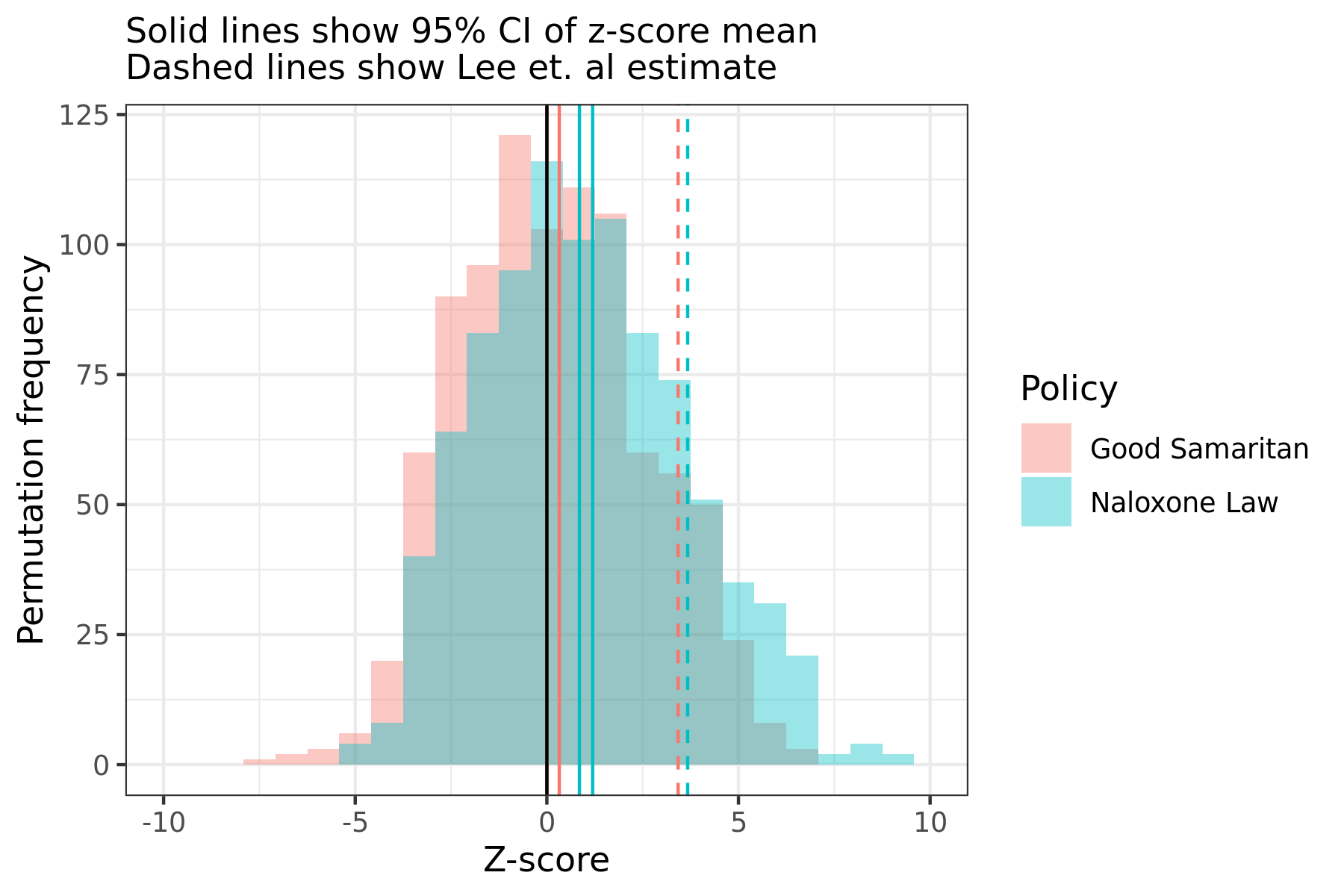

(i) REMA coef. std. error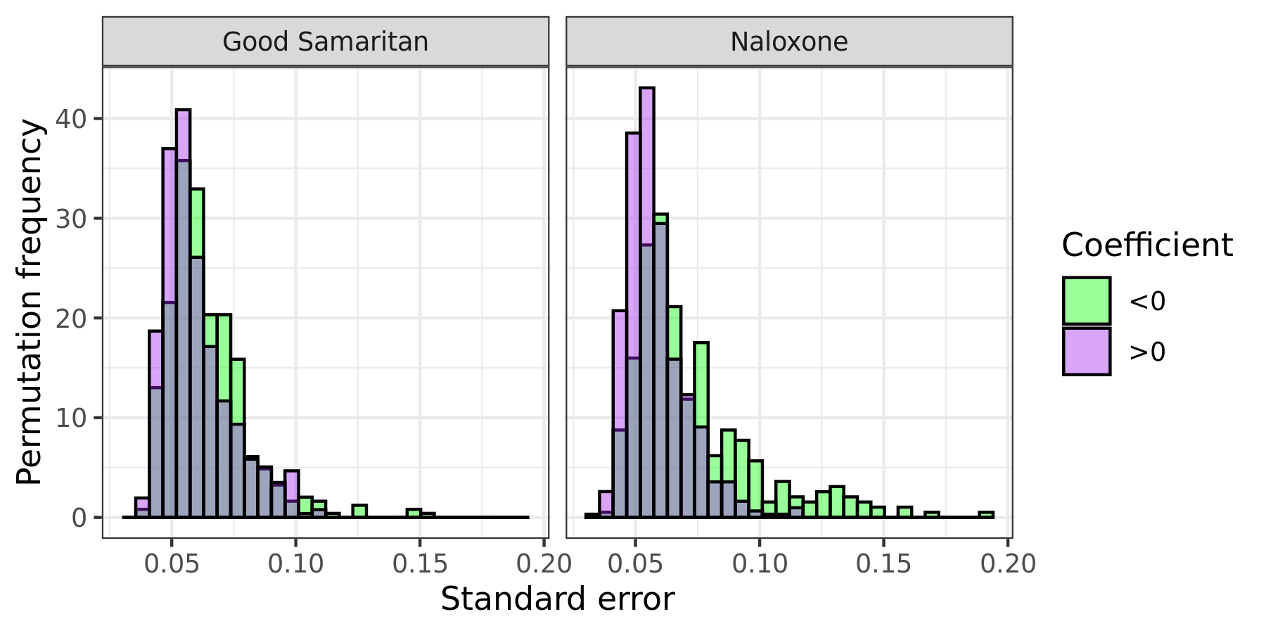

The distribution of z-scores also has tails that are too long and a right-ward bias for the individual coefficients of a given lead quarter (Figure 5B). A similar phenomenon in the standard errors can be seen on the quarterly lead level too.

Figure 5B: Z-score estimates from randomization of policy date for quarterly effect

The actual distribution of raw coefficient estimates under randomized policy dates is not as statistically problematic as the z-scores, since they are closer to being mean zero. However, even if the standard errors of the coefficient estimates were to be ignored and compared to the randomized policy date coefficient values, their p-values would be marginal, especially after an FDR correction was implemented (see Figure 5C). There would be no significant p-values for the Good Samaritan laws before adjustment, and a few for the Naloxone laws just under the 5% FDR cut-off (Q8, Q9-Q12). The REMA coefficients would be statistically insignificant after FDR correction, and all Good Samaritan coefficients would be as well even without a multiple comparisons adjustment.

Figure 5C: Permutation-based p-values

(6) Conclusion

The statistical estimates from Lee are compelling because of the size and quality of the dataset they use as well as the seeming appropriateness of the chosen statistical method. Though the matching method developed by Kim and Imai seem suited to the task of evaluating these policies and their effect on overdose deaths, econometric methods rely on numerous assumptions that are never fully met. Whether these violations amounts to a significant problem will depend with the quantity trying to be estimated. The econometric approach used in Lee is flawed because it leads to an over-rejection of the null hypothesis of no effect even when the date of policy adoption for Naloxone and Good Samaritan laws is randomized. Because the implication of the Lee paper would be significant if it informed policy, I strongly encourage revisions or adjustments to be made by the authors.

---

Notes