
A winner's curse adjustment for a single test statistic
Background
One of the primary culprits in the reproducability crisis in scientific research is the naive application of applied statistics for conducting inference. Even excluding cases of scientific misconduct, cited research findings are likely to be inaccurate due to 1) the file drawer problem, 2) researchers’ degrees of freedom and 3) underpowered statistical designs. To address the problem of publication bias some journals are now accepting findings regardless of their statistical significance. More than 200 journals now use the Open Science Foundation’s pre-registration framework to help improve reproducibility and reduce the garden of forking paths problem.
The frequentist paradigm is the dominant method for carrying out inference in scientific disciplines. This approach assumes that there exists a world of null hypotheses that are either true or false, and that all tests have an associated type-I and type-II error rate. This post will not discuss whether the frequentist paradigm is better or worse than the Bayesian one. Instead I will argue that the current practice of applied statistics fails to satisfy even its own principles as most disciplines focus solely on statistical significance (i.e. the type-I error rate). As a result the estimated power of a test is usually ignored or hastily calculated. For example in empirical economics the estimated median power across papers is a measly 18%. In biomedical research more attention is at least paid to power, but due to financial structures (e.g. the NIH requires power>80% for successful grants) researchers have an incentive to generate optimistic power estimates.
One consequence of using frequentist statistical tools to conduct scientific inference is that effect sizes will be biased when conditioned on statistical signifiance, even if the test itself is unbiased. This is because statistically significant findings have to be a certain number of standard deviations away from zero, and concomitantly certain values of the test are never observed (in the statistically significant space). The power-bias relationship helps to explain the Proteus phenomenon whereby follow-up studies tend to have a smaller effect size. The magnitude of this bias is known as the Winner’s Curse, and several adjustment procedures have been proposed in the context of multiple tests.[1] This is especially relevant in the field of genomics for polygenic risk scores developed with genome-wide association studies.
Many researchers who acknowledge the importance of power will explain their motivation in terms of rejecting false null hypotheses. This is important as a failure to a reject a null is a considered a “failed” experiment in the current world and therefore a waste of resources. But studies with high power are not only likely to be statistically significant they will also have effect sizes that are relatively accurate. Prioritizing power is one the main ways to address the reproducibility crisis because power and the effect size bias are inversely related.
In this post I will briefly review the frequentist paradigm that is used to conduct scientific inference and demonstrate how the probability of type-I and type-II errors are related to bias of significant effect sizes. In the final section of the post I propose a Winner’s Curse adjustment (WCA) procedure for a single test statistic. Note that Gelman and Carlin have also proposed an approach in their paper Beyond Power Calculations which suggests estimating the effect size bias and power prior to estimating the effect size and then using this information to assess the plausability of the observed result. My approach can be used in complement with theirs.
In summary this post will provide to explicit formulas for:
- The relationship between power and effect size bias \eqref{eq:power}
- An effect size deflator for single test statistic results \eqref{eq:deflator}
In the sections below the examples and math will be kept as simple as possible. All null and alternative hypothesis will come from a Gaussian distribution. Variances will be fixed and known. All hypothesis will be one-sided. Each of these assumptions can be relaxed without any change to the implications of the examples below, but do require a bit more math. Also note that \(\Phi\) refers to the standard normal CDF and its quantile function \(\Phi^{-1}\).
# modules used in the rest of the post
from scipy.stats import norm, truncnorm
import numpy as np
from numpy.random import randn
from scipy.optimize import minimize_scalar
import plotnine
from plotnine import *
import pandas as pd
(1) Review of Type-I and Type-II errors
Imagine a simple hypothesis test: to determine whether one Gaussian distribution, with a known variance, has a larger mean than another: \(y_{i1} \sim N(\mu_A, \sigma^2/2)\) and \(y_{i2} \sim N(\mu_B, \sigma^2/2)\), then \(\bar y_i \sim N(\mu_i, \sigma^2/n)\) and \(\bar d = \bar y_1 - \bar y_2 \sim N(\mu_A - \mu_B, \sigma^2/n)\). The sample mean (difference) will have a variance of \(\sigma^2/n\).[2]
\[\begin{align*} \bar d &\sim N(d, \sigma^2/n) \\ \bar z = \frac{\bar d - d}{\sigma / \sqrt{n}} &\sim N(0, 1) \end{align*}\]The null hypothesis is that: \(H_0: \mu_A \leq \mu_B\), with the alternative hypothesis that \(\mu_A > \mu_B\) (equivalent to \(d \leq 0\) and \(d >0\), respectively). Recall that in frequentist statistical paradigm, the goal is find a rejection region of the test statistic (\(z\)) that bounds the type-I error rate and maximizes power. When the null is true (\(d\leq 0\)) then setting \(c_\alpha = \Phi_{1-\alpha}^{-1}\), and rejecting the null when \(\bar z > c_\alpha\) will obtain a type-I error rate of exactly \(\alpha\).[3]
\[\begin{align*} P(\bar z > c) &\leq \alpha \\ 1-\Phi ( c ) &\leq \alpha \\ c &\geq \Phi^{-1}(1-\alpha) \end{align*}\]# EXAMPLE OF TYPE-I ERROR RATE
alpha, n, sig2, seed, nsim = 0.05, 18, 2, 1234, 50000
c_alpha = norm.ppf(1-alpha)
np.random.seed(1234)
err1 = np.mean([ (np.mean(randn(n)) - np.mean(randn(n)))/np.sqrt(2/n) > c_alpha for i in range(nsim)])
print('Empirical type-I error rate: %0.3f\nExpected type-I error rate: %0.3f' % (err1, alpha))
Empirical type-I error rate: 0.050
Expected type-I error rate: 0.050
In the event that the null is not true \((d > 0)\) then power of the test will depend four things:
- The magnitude of the effect (the bigger the value of \(d\) the better)
- The number of samples (the more the better)
- The type-I error rate (the larger the better)
- The magnitude of the variance (the smaller the better)
Defining the empirical test statistic as \(\bar z\), the type-II error rate is:
\[\begin{align*} 1 - \beta &= P( \bar z > c_\alpha) \\ 1 - \beta &= P\Bigg( \frac{\bar d - 0}{\sigma/\sqrt{n}} > c_\alpha \Bigg) \\ 1 - \beta &= P( z > c_\alpha - \sqrt{n} \cdot d / \sigma ) \\ \beta &= \Phi\Bigg(c_\alpha - \frac{\sqrt{n} \cdot d}{\sigma} \Bigg) \end{align*}\]# EXAMPLE OF TYPE-II ERROR RATE
d = 0.75
beta = norm.cdf(c_alpha - d / np.sqrt(2/n))
err2 = np.mean([ (np.mean(d + randn(n)) - np.mean(randn(n)))/np.sqrt(sig2 / n) < c_alpha for i in range(nsim)])
print('Empirical type-II error rate: %0.3f\nExpected type-II error rate: %0.3f' % (err2, beta))
Empirical type-II error rate: 0.274
Expected type-II error rate: 0.273
(2) Relationship between power and effect size bias
Most practitioners of applied statistics will be familiar with type-I and type-II error rates and will use these to interpret the results of studies and design trials. In most disciplines it is common that only statistically significant results (i.e. those ones that that reject the null) are analysed. In research domains where there are many hypothesis tests under consideration (such as genomics), multiple testing adjustments are made so that the number of aggregate false discoveries is bounded. Note that such adjustments are equivalent to increasing the value of \(c_\alpha\) and will lower the power of each test.
Unfortunately few researchers in my experience understand the relationship between power and effect size bias. Even though rigorously pre-specified research designs will likely have an accurate number of “true discoveries”, the distribution of significant effect sizes will almost certainly be overstated. An example will help to illustrate. Returning to the difference in Gaussian sample means, the distribution of statistically significant means will follow the following conditional distribution:
\[\begin{align*} \bar d^* &= \bar d | \bar z > c_\alpha \\ &= \bar d | \bar d > \sigma \cdot c_\alpha / \sqrt{n} \end{align*}\]Notice that the smallest observable and statistically significant mean difference will be at least \(c_\alpha\) root-\(n\) normalized standard deviations above zero. Because \(\bar d\) has a Gaussian distribution, \(\bar{d}^*\) has a truncated Gaussian distribution:
\begin{align}
\bar d^* &\sim TN(\mu, \sigma^2, l, u) \nonumber \\\
&\sim TN(d, \sigma^2 / n, \sigma \cdot c_\alpha / \sqrt{n}, \infty) \nonumber \\\
a &= \frac{l - \mu}{\sigma} = c_\alpha - \sqrt{n}\cdot d / \sigma = \Phi^{-1}(\beta) \nonumber \\\
E[\bar d^*] &= d + \frac{\phi(a)}{1 - \Phi(a)} \cdot (\sigma/\sqrt{n}) \nonumber \\\
&= d + \underbrace{\frac{\sigma \cdot \phi(\Phi_\beta^{-1})}{\sqrt{n}(1 - \beta)}}_{\text{bias}} \tag{1}\label{eq:power}
\end{align}
The bias of the truncated Gaussian is shown to be related to a handful of statistical parameters including the power of the test! The bias can also be expressed as a ratio of the mean of the statistically significant effect size to the true one, what I will call the bias ratio,
\[\begin{align*} \text{R}(\beta;n,d,\sigma) &= \frac{E[\bar d^*]}{d} = 1 + \frac{\sigma \cdot \phi(\Phi_\beta^{-1})}{d\cdot\sqrt{n}\cdot(1 - \beta)} \end{align*}\]where \(\beta = f(n,d,\sigma)\), and \(R\) is ultimately a function of the sample size, true effect size, and measurement error. The simulations below show the relationship between the bias ratio and power for different effect and sample sample sizes.
def power_fun(alpha, n, mu, sig2):
  thresh = norm.ppf(1-alpha)
  t2_err = norm.cdf(thresh - mu/np.sqrt(sig2/n))
  return 1 - t2_err
  return

def bias_ratio(alpha, n, mu, sig2):
  power = power_fun(alpha=alpha, n=n, mu=d, sig2=sig2)
  num = np.sqrt(sig2) * norm.pdf(norm.ppf(1-power))
  den = mu * np.sqrt(n) * power
  return 1 + num / den

# SIMULATE ONE EXAMPLE #
np.random.seed(seed)
nsim = 125000
n, d = 16, 0.5
holder = np.zeros([nsim, 2])
for ii in range(nsim):
  y1, y2 = randn(n) + d, randn(n)
  dbar = y1.mean() - y2.mean()
  zbar = dbar / np.sqrt(sig2 / n)
  holder[ii] = [dbar, zbar]

emp_power = np.mean(holder[:,1] > c_alpha)
theory_power = power_fun(alpha=alpha, n=n, mu=0.5, sig2=sig2)
emp_ratio = holder[:,0][holder[:,1] > c_alpha].mean() / d
theory_ratio = bias_ratio(alpha, n, d, sig2)
print('Empirical power: %0.2f, theoretical power: %0.2f' % (emp_power, theory_power))
print('Empirical bias-ratio: %0.2f, theoretical power: %0.2f' % (emp_ratio, theory_ratio))

# CALCULATE CLOSED-FORM RATIO #
n_seq = np.arange(1,11,1)**2
d_seq = np.linspace(0.01,1,len(n_seq))

df_ratio = pd.DataFrame(np.array(np.meshgrid(n_seq, d_seq)).reshape([2,len(n_seq)*len(d_seq)]).T, columns=['n','d'])
df_ratio.n = df_ratio.n.astype(int)
df_ratio = df_ratio.assign(ratio = lambda x: bias_ratio(alpha, x.n, x.d, sig2),
                           power = lambda x: power_fun(alpha, x.n, x.d, sig2))

gg_ratio = (ggplot(df_ratio, aes(x='power',y='np.log(ratio)',color='n')) +
            geom_point() + theme_bw() +
            ggtitle('Figure 1: Relationship between power and effect size bias') +
            labs(x='Power',y='log(Bias Ratio)') +
            scale_color_gradient2(low='blue',mid='yellow',high='red',midpoint=50,
                                  name='Sample Size'))
plotnine.options.figure_size = (5,3.5)
gg_ratio
Empirical power: 0.41, theoretical power: 0.41
Empirical bias-ratio: 1.67, theoretical power: 1.67
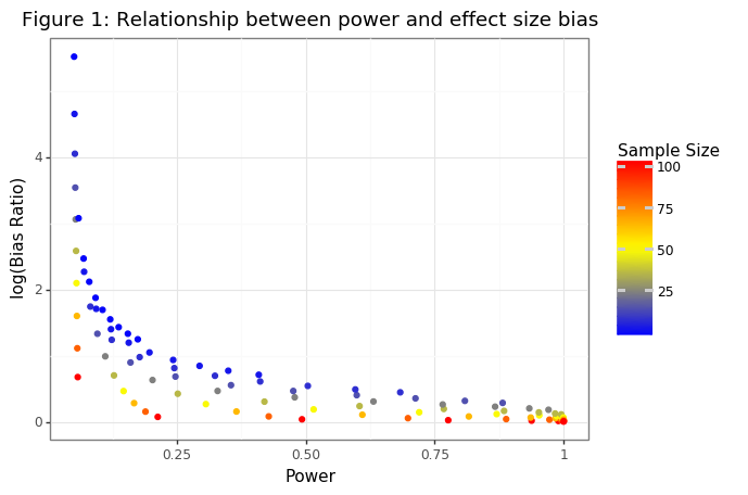
Figure 1 shows that while there is not a one-to-one relationship between the power and the bias ratio, generally speaking the higher the power the lower the ratio. The variation in low powered tests is driven by the sample size. Tests that have low power because they have a large sample sizes but small effect size will have a much smaller bias than equivalently powered tests with large effect sizes and small sample sizes. The tables below highlight this fact by showing the range in power for tests with similar bias ratios, the range in bias ratios for similarly powered tests.
np.round(df_ratio[(df_ratio.ratio > 1.3) & (df_ratio.ratio < 1.4)].sort_values('power').head(),2)
| n | d | ratio | power |
|---|---|---|---|
| 64 | 0.12 | 1.33 | 0.17 |
| 49 | 0.23 | 1.31 | 0.31 |
| 36 | 0.34 | 1.36 | 0.42 |
| 25 | 0.56 | 1.36 | 0.63 |
| 25 | 0.67 | 1.30 | 0.77 |
np.round(df_ratio[(df_ratio.power > 0.45) & (df_ratio.power < 0.52)].sort_values('ratio').head(),2)
| n | d | ratio | power |
|---|---|---|---|
| 100 | 0.23 | 1.04 | 0.49 |
| 49 | 0.34 | 1.21 | 0.52 |
| 25 | 0.45 | 1.45 | 0.48 |
| 16 | 0.56 | 1.60 | 0.48 |
| 9 | 0.78 | 1.73 | 0.50 |
(3) Why estimating the bias of statistically significant effects is hard!
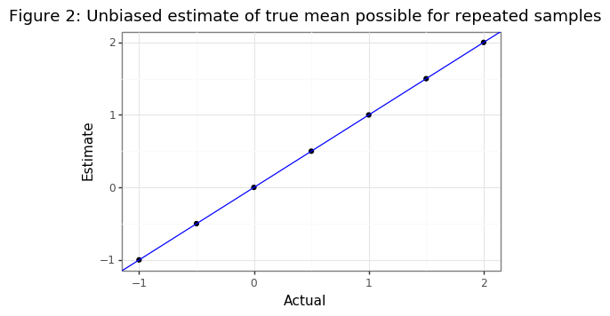
If the true effect size were known, then it would be possible to explicitly calculate the bias term. Unfortunately this parameter is never known in the real world. If there happened to be multiple draws from the same hypothesis then an estimate of the true mean could be found. With multiple draws, there will be an observed distribution of \(\bar{d}^*\) so that the empirical mean \(\hat{\bar{d}}^*\) could be used by optimization methods to estimate \(d\) using the formula for the mean of a truncated Gaussian.
\[\begin{align} d^* &= \arg\min_d \hspace{2mm} \Bigg[ \hat{\bar d}^* - \Bigg( d + \frac{\phi(c_\alpha-\sqrt{n}\cdot d/\sigma)}{1 - \Phi(c_\alpha-\sqrt{n}\cdot d/\sigma)} \cdot (\sigma/\sqrt{n}) \Bigg) \Bigg]^2 \tag{2}\label{eq:MLE} \end{align}\]The simulations below show that with enough hypothesis rejections, the true value of \(d\) could be determined. However if the null could be sampled multiple times then the exact value of \(d\) could be determined by just looking at \(\bar d\)! The code is merely to highlight the principle.
def mu_trunc(mu_true, alpha, n, sig2):
  sig = np.sqrt(sig2 / n)
  a = norm.ppf(1-alpha) - mu_true / sig
  return mu_true + norm.pdf(a)/(1-norm.cdf(a)) * sig

def mu_diff(mu_true, mu_star, alpha, n, sig2):
  diff = mu_star - mu_trunc(mu_true, alpha, n, sig2)
  return diff**2

def mu_find(mu_star, alpha, n, sig2):
  hat = minimize_scalar(fun=mu_diff,args=(mu_star, alpha, n, sig2),method='brent').x
  return hat

n = 16
nsim = 100000

np.random.seed(seed)
d_seq =  np.round(np.linspace(-1,2,7),1)
res = np.zeros(len(d_seq))
for jj, d in enumerate(d_seq):
  holder = np.zeros([nsim,2])
  # Generate from truncated normal
  dbar_samp = truncnorm.rvs(a=c_alpha-d/np.sqrt(sig2/n),b=np.infty,loc=d,scale=np.sqrt(sig2/n),size=nsim,random_state=seed)
  z_samp = dbar_samp / np.sqrt(sig2/n)
  res[jj] = mu_find(dbar_samp.mean(), alpha, n, sig2)

df_res = pd.DataFrame({'estimate':res, 'actual':d_seq})

plotnine.options.figure_size = (5.5, 3.5)
gg_res = (ggplot(df_res, aes(y='estimate',x='actual')) + geom_point() +
         theme_bw() + labs(y='Estimate',x='Actual') +
         geom_abline(intercept=0,slope=1,color='blue') +
         ggtitle('Figure 2: Unbiased estimate of true mean possible for repeated samples'))
gg_res
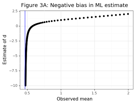
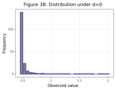
But if multiple samples are unavailable to estimate \(\hat{\bar{d}}^*\), then can the value of \(d\) ever be estimated? A naive reproach using only a single value to find \(d^*\) via an MLE approach of equation \eqref{eq:MLE} yields negative estimates when \(\mu \approx 0\) because many values below the median of the truncated normal with a small mean have will match a large and negative mean for another truncated normal. Figures 3A and 3B show this asymmetric phenomenon.
n = 25
sig, rn = np.sqrt(sig2), np.sqrt(n)
d_seq = np.linspace(-10,2,201)
df1 = pd.DataFrame({'dstar':d_seq,'d':[d + norm.pdf(c_alpha - rn*d/sig) / norm.cdf(rn*d/sig - c_alpha) * (sig/rn) for d in d_seq]})
sample = truncnorm.rvs(c_alpha, np.infty, loc=0, scale=sig/rn, size=1000, random_state=seed)
df2 = pd.DataFrame({'d':sample,'tt':'dist'})
plotnine.options.figure_size = (5,3.5)
plt1 = (ggplot(df1,aes(y='dstar',x='d')) + geom_point() + theme_bw() +
        geom_vline(xintercept=c_alpha*sig/rn,color='blue') +
        labs(x='Observed mean',y='Estimate of d') +
        ggtitle('Figure 3A: Negative bias in ML estimate'))
plt2 = (ggplot(df1,aes(x='d')) + theme_bw() +
geom_histogram(fill='grey',color='blue',bins=30) +
labs(x='Observed value',y='Frequency') +
ggtitle('Figure 3B: Distribution under d=0'))
plt1
pl2
(4) Approaches to de-biasing single-test statistic results
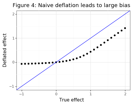
A conservative method to ensure that \(E[ \bar{d}^* -d ] \leq 0\) when \(d\geq 0\) is to subtract off the bias when the null is zero: \((\sigma \cdot \phi(c_\alpha)) / (\sqrt{n}\cdot\Phi(-c_\alpha))\). The problem with this approach is that for true effect (\(d>0\)), the bias estimate will be too large and the estimate of the true effect will actually be too small as Figure 4 shows.
d_seq = np.linspace(-1,2,31)
bias_d0 = norm.pdf(c_alpha)/norm.cdf(-c_alpha)*np.sqrt(sig2/n)
df_bias = pd.DataFrame({'d':d_seq,'deflated':[mu_trunc(dd,alpha,n,sig2)-bias_d0 for dd in d_seq]})

plotnine.options.figure_size = (5,3.5)
gg_bias1 = (ggplot(df_bias,aes(x='d',y='deflated')) + theme_bw() +
            geom_point() + labs(x='True effect',y='Deflated effect') +
            geom_abline(intercept=0,slope=1,color='blue') +
            scale_x_continuous(limits=[min(d_seq),max(d_seq)]) +
            scale_y_continuous(limits=[min(d_seq),max(d_seq)]) +
            ggtitle('Figure 4: Naive deflation leads to large bias'))
gg_bias1
A better approach I have devised is to weight the statistically significant observation by where it falls in the cdf of truncated Gaussian for \(d=0\). When \(d>0\) most \(\bar{d}^*\) will be above this range and receive little penalty, whereas for values of \(d \approx 0\) they will tend to receive a stronger deflation.
\[\begin{align} b_0 &= \frac{\sigma}{\sqrt{n}} \frac{\phi(c_\alpha)}{\Phi(-c_\alpha)} = \text{bias}(\bar d^* | d=0) \nonumber \\ d^* &= \bar d^* - 2\cdot[1 - F_{\bar d>c_\alpha\sigma/\sqrt{n}}(\bar d^*|d=0)] \cdot b_0 \tag{3}\label{eq:deflator} \end{align}\]The simulations below implement the deflation procedure suggested by equation \eqref{eq:deflator} for a single point estimate for different sample and effect sizes.
nsim = 10000

di_cn = {'index':'tt','25%':'lb','75%':'ub','mean':'mu'}
d_seq = np.linspace(-0.5,1.5,21)
n_seq = [16, 25, 100, 250]

holder = []
for n in n_seq:
  bias_d0 = norm.pdf(c_alpha)/norm.cdf(-c_alpha)*np.sqrt(sig2/n)
  dist_d0 = truncnorm(a=c_alpha,b=np.infty,loc=0,scale=np.sqrt(sig2/n))
  sample_d0 = dist_d0.rvs(size=nsim, random_state=seed)
  w0 = dist_d0.pdf(sample_d0).mean()
  sim = []
  for ii, d in enumerate(d_seq):
    dist = truncnorm(a=c_alpha-d/np.sqrt(sig2/n),b=np.infty,loc=d,scale=np.sqrt(sig2/n))
    sample = dist.rvs(size=nsim, random_state=seed)
    deflator = 2*(1-dist_d0.cdf(sample))*bias_d0
    # deflator = dist_d0.pdf(sample)*bias_d0 / w0
    d_adj = sample - deflator
    mat = pd.DataFrame({'adj':d_adj,'raw':sample}).describe()[1:].T.reset_index().rename(columns=di_cn)[list(di_cn.values())].assign(d=d,n=n)
    sim.append(mat)
  holder.append(pd.concat(sim))
df_defl = pd.concat(holder)

plotnine.options.figure_size = (9,6)
gg_bias2 = (ggplot(df_defl,aes(x='d',y='mu',color='tt')) + theme_bw() +
            geom_linerange(aes(ymin='lb',ymax='ub',color='tt')) +
            geom_point() + labs(x='True effect',y='Observed statistically significant effect') +
            geom_abline(intercept=0,slope=1,color='black') +
            geom_vline(xintercept=0, linetype='--') +
            scale_x_continuous(limits=[-0.75,1.8]) +
            scale_y_continuous(limits=[-0.75,1.8]) +
            facet_wrap('~n', labeller=label_both) +
            scale_color_discrete(name='Type',labels=['Deflated','Observed']) +
            ggtitle('Figure 5: Deflating by the cdf of d=0 achieves better results\nVertical lines show IQR'))
gg_bias2
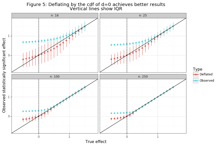
Figure 5 shows that the bias for values of \(d \geq 0\) is now conservative and limited. Especially for larger samples, a large and otherwise highly significant effect will be brought much closer to its true value. The primary drawback to using the WCA from equation \eqref{eq:deflator} is that it adds further noise to the point estimate. While this is statistically problematic, from an epistemological viewpoint it could be useful to reduce the confidence of researchers in their “significant” findings that are unlikely to replicate at an equivalent level.
(5) Summary
WCAs for single test results are much more challenging that those for repeated test measurements due to a lack of measured information. I have proposed a simple formula \eqref{eq:deflator} that can be used on all statistically significant results requiring only the observed effect size, type-I error rate, sample size, and noise estimate. For small to medium sample sizes this deflator leads to additional noise in the point estimate, but may reduce exaggerated effect sizes seen in the literature. While it has no doubt been expressed before, I also derive the analytical relationship between power and effect size bias \eqref{eq:power}.
As a final motivating example consider the well-regarded paper Labour Market Returns to Early Childhood Stimulation by Gertler et. al (2013) which includes a Nobel-prize winning economist in its author list. I am borrowing this example from an Andrew Gelman discussion paper. The Gertler paper claims to show that an educational intervention using a randomized control trial improved long-run income earnings by 42%. This is a huge increase as the author’s note: “[t]hese findings show that psychosocial stimulation early in childhood in disadvantaged settings can have substantial effects on labour market outcomes and reduce later life inequality”.”
The results … show that the impact on earnings remains large and statistically significant
As this post has discussed, it is quite likely that they should have said these results are statistically significant because they were large. For the main effect, Table 3 in the paper shows a p-value for 0.01 a sample size of 105, implying that \(1 - \Phi(0.42/(1.9/\sqrt{105})) \approx 0.01\), with a z-score of around 2.7. The code below shows that if there were no effect, then the average statistically significant effect that would be observed would be 0.372 (note that the median bias would be lower because of the right-skew of the truncated normal distribution). However because the result (42%) is in the 80th percentile of such a distribution, the adjustment procedure suggests removing only 15% off of the point estimate. Using a WCA adjustment for this paper reduces the findings to 27%, which is still quite high and respectable. I hope this post will help to raise awareness of of how the Winner’s Curse affects applied statistical research.
alpha = 0.05
c_alpha = norm.ppf(1-alpha)
dstar = 0.42
sig2 = 1.85**2
n = 105
bias_d0 = norm.pdf(c_alpha)/norm.cdf(-c_alpha)*np.sqrt(sig2/n)
dist_d0 = truncnorm(a=c_alpha,b=np.infty,loc=0,scale=np.sqrt(sig2/n))
adj = 2*(1-dist_d0.cdf(dstar))*bias_d0

print('Baseline effect: %0.3f, P-value: %0.3f\nBias when d=0: %0.3f\nDeflator: %0.3f\nAdjusted effect: %0.3f' %
      (dstar, 1-norm.cdf(dstar/np.sqrt(sig2/n)),bias_d0, adj, dstar - adj))
Baseline effect: 0.420, P-value: 0.010
Bias when d=0: 0.372
Deflator: 0.149
Adjusted effect: 0.271
Footnotes
-
Note that the Winner’s Curse in economics is a different but related phenomenon. ↩
-
If the variances were unknown, then the difference in means would have a student-t distribution with slightly fatter tails. ↩
-
If \(c > c_\alpha\), then the type-I error rate would be lower (which is good), but, the power would also be lower in the event that the null were false. It is therefore desirable the rejection region obtain the exactly desired type-I error rate, and then the statistician can decide what type-I level to choose. ↩