Background

Twenty years ago Tibshirani developed a penalized regression model known as the Lasso. Instead of using the L0-norm as the penalty term (equivalent to best-subset selection), the Lasso makes use of an L1-norm. This subtle change in norms has several important properties including a model which allows for both regularization and model selection,[¹] and the use of state-of-the-art optimization algorithms such as coordinate descent that allows the Lasso to scale to large \(p\) datasets.

The coefficient vector of the Lasso is found by minimizing some convex loss function plus the L1-norm of the coefficients weighted by \(\lambda\), as equation \eqref{eq:lasso1} shows. This simple formulation can and has been extended, and there is now a large family of Lasso-based estimators including the elastic net, group Lasso, fused Lasso estimators, \(\sqrtl\), and many others.

The choice of \(\lambda\) is crucial in determining the performance of the Lasso estimator. Too small a value leads a coefficient vector too-similar to least-squares leading to unacceptably high variance; and too large a value leads to a model with substantial bias. When the statistical learning task is simply to maximize generalization error, cross-validation can be employed. Alternatively, information-theoretic approaches (AIC/BIC/Stein’s) can also be used, although these approaches are not exactly tailored for the Lasso.[²]

Are there any alternative approaches to selecting \(\lambda\) besides the two previously mentioned routes? The answer is yes, and it is largely thanks to the theoretical work of high-dimensional statistics which has flourished over the last decade. The recently published Statistical Learning with Sparsity (SLWS) represents a landmark text in the field. This post will consider how some simple theoretical properties of the Lasso allow for a disciplined choice of the regularization parameter that avoid traditional tuning approaches. There are three subsequent sections: (1) a discussion of how prediction bounds in the Lasso can be established by a specific choice of regularization parameter, (2) how the \(\sqrtl\) leverages these properties to provide an estimator that is invariant to Gaussian noise levels, and (3) an applied example on high-dimensional microarray data for 21 cancer types.

In addition to SLWS, this post was heavily informed by Belloni’s lectures.

(1) Some statistical properties of the Lasso

Throughout this post a simple homoskedastic regression data generating process (DGP) will be assumed with a response vector \(\text{len}(\by)=N\) and a \(p\)-dimensional feature matrix \(\text{dim}(X)=p\).

Least-squares case

Before considering the Lasso, the more simply least squares model is useful for some building intuition. When \(N>p\), the least-squares solution to fitting the data to this problem has the following closed-form solution: \(\hat{\bbeta} = \arg \min_{\beta} \|\by - \bX\bbeta \|_2^2 = (\bX^T\bX)^{-1}\bX^T\by\). In order to establish prediction bounds for this estimator, one begins by writing down the optimality conditions.

The first line just states that since \(\bbetah\) is the optimal solution, no other coefficient vector, including the true coefficient vector \(\bbetaz\) can achieve a lower mean-squared error (for a given realization of the DGP). The left-hand side of equation \eqref{eq:pred_ols1} is the mean-squared prediction norm error (MSPNE) which is the term of interest: it measures how close an estimated model is to the true linear predictor.[³] Furthermore, one can see that on the right-hand side of equation \eqref{eq:pred_ols1} the MSPNE is bounded by a bias and a variance term in the L2-norms. Specifically, the noisier the relationship between the columns of \(\bX\) and the error term is, and the larger the euclidean distance of \(\bbetah\) to \(\bbetaz\), the higher the prediction norm error will be. Of course the least squares model cannot actually trade-off between these two terms.

To further explore the prediction bounds, we need to perform the following inequality decomposition:

Where \(\Lambda(\cdot)\) refers to the eigenvalue of the matrix. The first property is derived from showing that \(E(\| \bX^T \be \|_2^2)=\sigma^2 \text{tr}(\bX^T\bX) \leq \sigma^2 \cdot p \cdot \Lambda_{\max}(\bX^T\bX)\) and then applying a Chebyshev-bound, and the second is more complicated but a justification can be found Sara van de Geer’s works.

The resulting root-\(N\) prediction norm error bound shown in equation \eqref{eq:pred_ols2} is highly intuitive since it says that the scale of the error that converges to zero at a rate of \(\sqrt{N}\) is proportional to: (i) the standard-deviation of error \(\sigma\), (ii) design matrix conditions (\(\Lambda_{\max}/\Lambda_{\min}\)), and (iii) ratio of features to observations (\(p/N\)). The ratio of the largest to the smallest eigenvalue indicates whether the features are orthogonal to each other or contain repetitive information (think PCA). Naturally, the more features there are to observations, the fewer the effective degrees of freedom there will be and the fit will worsen.

Lasso case

There are several ways to think about why the least-squares prediction bound breaks down in the high-dimensional case (\(p \gg N\)). Most obviously, the gram-matrix becomes non-full rank \(\Lambda_{\min}(\gram)=0\). Alternatively we can identify part of the problem with the L2 norms such that the variance term \(\be^T\bX\) cannot be sufficiently bounded. This is where the use of infinity norms can be leveraged under the Lasso case.[⁴]

Going forward, we’re going to assume that the model is both high-dimensional and sparse: \(\|\beta_0 \|_0=s \ll N\), \(\text{dim}(\beta_0)=p \gg N\), and denote the true model index \(T=\text{supp}(\beta_0) \subseteq {1,\dots,p }\). In other words, even though our design matrix has \(p\) features (which exceed the observation count), we assume that only \(s\) of them are actually causally relevant. As before, we start with optimality conditions:

Before we broke down the error term with Cauchy-Schwartz (\(|\langle u,v \rangle|\leq \|u\|_2\|v\|_2\)) but now we will use Holder’s inequality (\(\|u\cdot v\|_1\leq \|u\|_p\|v\|_q\) where \(1/p+1/q=1\)) to achieve the desired infinity-norm.

It turns out that one can think of \(\| \bX^T \be \|_{\infty}\) as the variance term, and if \(\lambda\) is chosen to moderate this term at the expense of \(\| \hat{\beta}-\beta_0 \|_1\) (bias) a prediction bound can be achieved. Therefore define the event: \(E = \Big\{\lambda \geq c \frac{\| \bX^T \be \|_{\infty}}{N}\Big\}, \hspace{2mm} c>1\), set \(\lambda\) s.t. \(P(E)\to 1\) as \(N \to \infty\) Assuming that event \(E\) holds:

Next, we introduce the restricted eigenvalue condition:

Continuing on:

So we get a nice:

This leads to the question of how to get \(\lambda \geq c \frac{\|\bX^Te\|_\infty}{N}\). For a discussion of the restricted eigenvalue condition, see Chapter 11 of SLWS. Assuming that \(\bX\) has been normalized, and the variance of the error is known, we can pick \(\lambda\) so that event \(E\) holds with probability at least \(1-\alpha\):

Substituting \(\lambda^*\) back into the prediction norm gives:

This is an extremely elegant result. Notice the similarities between equations \eqref{eq:pred_ols2} and \eqref{eq:pred_lasso1}, and that the Lasso now has a very similar prediction bound to the least squares case. In other words, one doesn’t pay too much in terms of prediction error by the use of an L1 penalty norm. However, the choice of \(\lambda\) in equation \eqref{eq:lam1} required knowledge of \(\sigma\)! While the variance of the error term can of course be estimated, there are few guarantees for its accurate reconstruction in a high-dimensional setting. However, as the next section shows, a modification of the Lasso problem can avoid this problem.

(2) Statistical properties of the SQRT-Lasso

Recalling the steps of how \(\lambda^*\) was chosen, its easy to see that for a different loss function, the general choice of \(\lambda\) for the selection event is: \(\lambda > c \|-\nabla \ell(\bbetaz;\bX)\|_\infty\). In other words, we need \(\lambda\) to exceed the largest absolute value of the gradient under the true model. This represents the magnitude of the noise we want to moderate with the regularization term. The \(\sqrtl\) is a simple modification to the Lasso optimization problem: use the square-root of the loss function rather than the mean-squared error (MSE) [Belloni et al 2011]. This seemingly-trivial modification leads to a gradient whose infinity-norm is pivotal to the underlying variance structure.

In other words, the distribution of the gradient of the \(\sqrtl\) under the true coefficient vector is stochastically identical regardless of the magnitude of \(\sigma^2\)! More amazingly, any given component of the this gradient has a student-t distribution!

Where \(\Phi_t^{-1}\) is the quantile of the student-t with \(N\) degrees of freedom. This makes choosing \(\lambda\) so that event \(E\) holds with probability at least \(1-\alpha\) very easy, since the choice is just a function \(\alpha\) and \(p\) as equation \eqref{eq:lam2} shows. Because the loss-function of the \(\sqrtl\) is a monotonic transformation of a convex loss function, it is also convex. More impressively, the coordinate descent update for \(\sqrtl\) also has a closed-form solution. It’s interesting to compare the two coordinate updates between the algorithms.

Coordinate descent algorithms

While the update term for the \(\sqrtl\) is more complicated, the key point is that it keeps track of the the sum of squared residuals, and therefore a measure of the variance of the error. Let’s run some simulations to see how well the models do in the high-dimensional and sparse case. We’ll assume the following set-up: \(\sigma^2=2\), \(N=100\), \(p=1000\), \(s=5\), where \(\bbetaz={\underbrace{1,\dots,1}_{\times 5},\underbrace{0,\dots,0}_{\times 995}}\). Four baseline models will be considered: (i) \(\lambda\)’s chosen to minimizes the loss function (CV-min) on the hold-out folds as well as (ii) the most conservative \(\lambda\) whose out-of-fold loss is within one standard deviation of the minimum (CV-1se), (iii) a \(\lambda\) chosen from equation \eqref{eq:lam1} where we somehow “know” the true variance (Lasso-theory), and (iv) the \(\sqrtl\) with \(\lambda\) from equation \eqref{eq:lam2} (Lasso-SQRT). Furthermore, both the Lasso-theory and Lasso-SQRT will also include a least-squares and CV-tuned Ridge regression model whereby the index of non-zero coefficients is used to re-estimate the model.

Three metrics will be considered:

1. The receiver operator characteristic (ROC): i.e. the number of true positives (TPs) and false positives (FPs) selected by each model sensitivity/specificity
2. The accuracy of reconstructing \(\bbetaz\): \(\|\bbetah_T - \bbetaz \|_1\), and well as it’s error: \(\|\bbetah_{T^C}\|_1\)
3. The generalization error, measured in MSE to see how well each manages the bias/variance trade-off

Figure 1: Simulation results

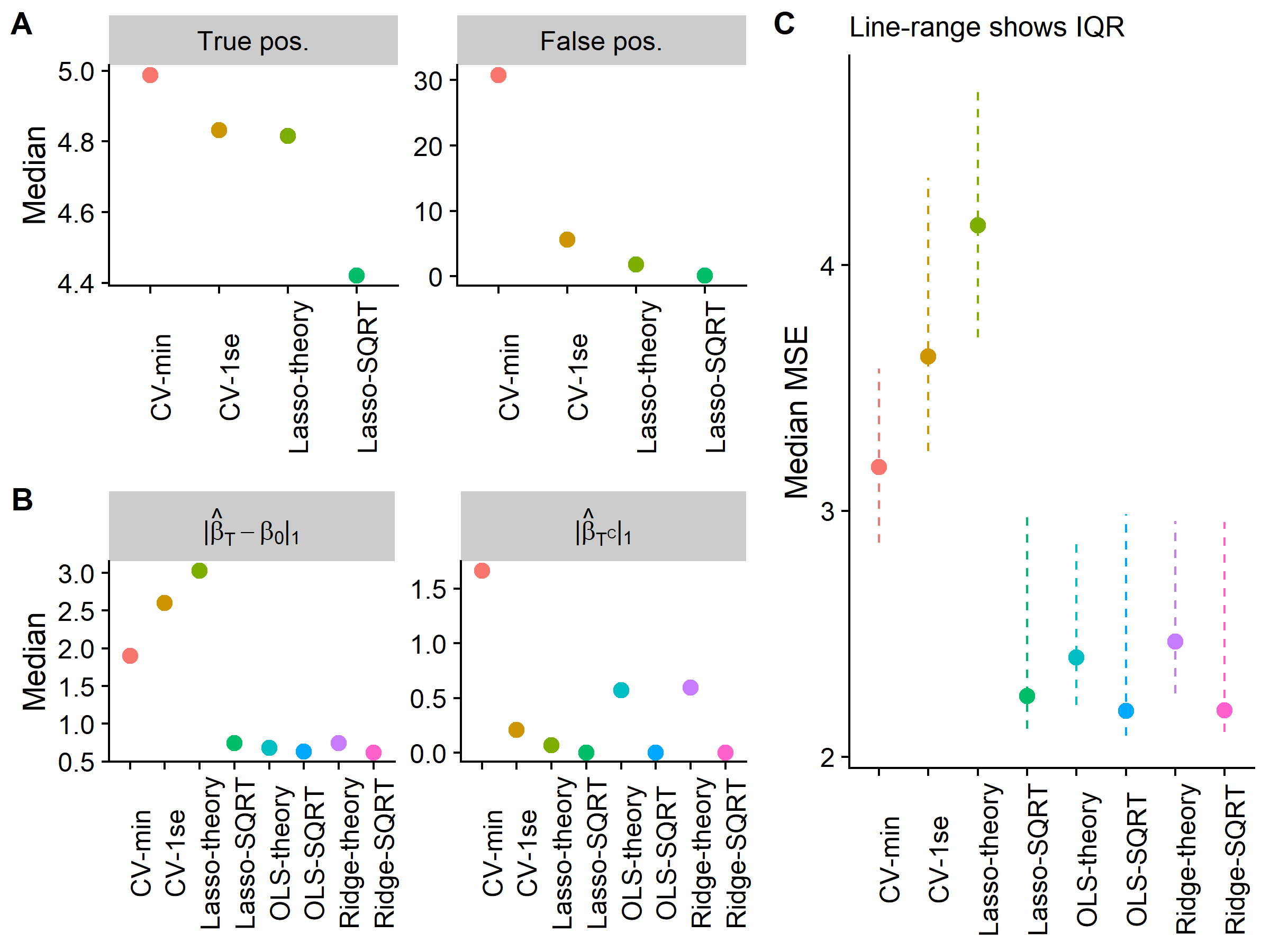
Figure 1A shows that each estimator is able to select most of the true features, most of the time, although the \(\sqrtl\) has the worst sensitivity with a median of 4.4 out of 5. However, the \(\sqrtl\) almost never selects false positives making it a less noisy estimator. In contrast, the CV-min selects 30 noise features! This reveals why the \(\sqrtl\) or the Lasso-theory approaches are well suited to post-estimation with either least-squares or ridge regression because they select a small number of features that will tend to be right ones.

Figure 1B shows that the OLS/Ridge post-estimators do very well in reconstructing \(\bbetaz\), although the \(\sqrtl\)’s post-estimators are better in terms of avoiding assigning the coefficient budget towards the noise variables. Lastly, in Figure 1C we see that the \(\sqrtl\) and its post-estimators achieve the smallest MSE revealing the advantage of this theoretically motivated choice over the common paradigm of cross-validation.

A discerning reader might point out that this approach nevertheless still assumes that the error is Gaussian. This does not turn out to be a significant problem because even if \(|\bX_j^T \be| / \|\be \|_2\) is non-Gaussian, it is characterized by self-normalized process,[⁵] and will have a distribution which will be well-approximated by the student-t anyways, especially in the tails of the distribution. The skeptical may find a simulation to be more convincing.

n=p=100
set.seed(1)
sn.sims <- replicate(250,{
X <- scale(matrix(rexp(n*p),ncol=p)) # Non-gaussian design matrix
e1 <- rnorm(n) # Gaussian error
e2 <- rnorm(n,sd=sqrt(abs(apply(X,1,sum)))) # Heteroskedastic error
e3 <- rexp(n)-1 # Exponential (mean zero)
sn1 <- abs(as.vector(t(X) %*% e1))/sqrt(sum(e1*e1))
sn2 <- abs(as.vector(t(X) %*% e2))/sqrt(sum(e2*e2))
sn3 <- abs(as.vector(t(X) %*% e3))/sqrt(sum(e3*e3))
sapply(list(sn1,sn2,sn3),quantile,p=0.99)
})
sn.df <- data.frame(t(sn.sims))
colnames(sn.df) <- c('Homoskedastic','Heteroskedastic','Exponential')
sn.df <- gather(sn.df)
 
# Plot with ggplot!

Figure 2: Self-normalizing sums

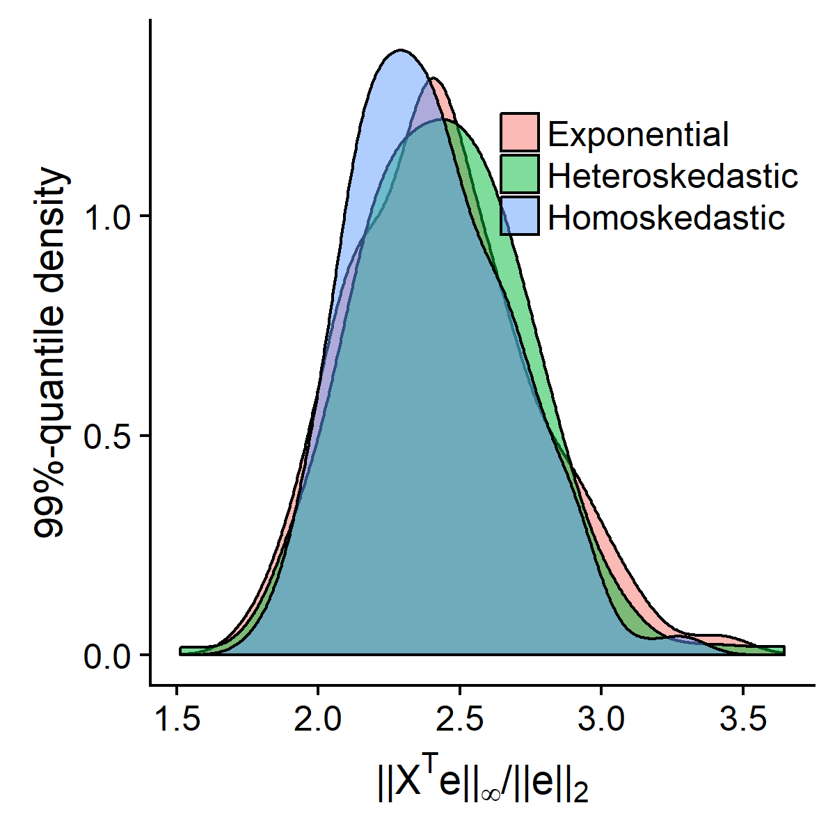
One significant problem with the choice of \(\lambda\) in equation \eqref{eq:lam2} for the \(\sqrtl\) is that it is a conservative estimate because it assumes the upper bound situation where the columns of the design matrix are orthogonal to each other. In reality, there will almost surely be some correlation between the features and a lower \(\lambda\) will be needed to prevent too much bias. While the distribution of the error term is unknown, we’ve already shown that the event target can be approximated by a self-normalizing sum from the standard normal case. This allows for a choice of \(\lambda\) to closely match the actual quantile of \(\|\bX^T \be \|_\infty / \|\be \|_2\).

In the next section when genomic data is employed, the data-driven choice of \(\lambda^*\) from equation \eqref{eq:lam3} will be used.

(3) Application to microarray data

To test out how well \(\sqrtl\) compares to the benchmark CV-tuned Lasso estimator on real data, we will use randomly selected gene expression measurements from the datamicroarray package. This package has 22 microarray datasets with 13 cancer types including breast cancer, leukemia, and and prostate cancer. The number of observations ranges from 31 to 248, whereas the feature size ranges from 456 to 54613. The average ratio of \(p/N\) is 140, making these datasets very high-dimensional and good testing grounds for the \(\sqrtl\). The table below provides more information.

##         author year   N     p              Disease
## 1         Alon 1999  62  2000         Colon Cancer
## 2    Borovecki 2005  31 22283 Huntington's Disease
## 3   Burczynski 2006 127 22283      Crohn's Disease
## 4    Chiaretti 2004 111 12625             Leukemia
## 5         Chin 2006 118 22215        Breast Cancer
## 6     Chowdary 2006 104 22283        Breast Cancer
## 7  Christensen 2009 217  1413                  N/A
## 8        Golub 1999  72  7129             Leukemia
## 9       Gordon 2002 181 12533          Lung Cancer
## 10     Gravier 2010 168  2905        Breast Cancer
## 11        Khan 2001  63  2308                SRBCT
## 12    Nakayama 2001 105 22283              Sarcoma
## 13     Pomeroy 2002  60  7128            CNS Tumor
## 14       Shipp 2002  58  6817             Lymphoma
## 15       Singh 2002 102 12600      Prostate Cancer
## 16      Sorlie 2001  85   456        Breast Cancer
## 17          Su 2002 102  5565                  N/A
## 18 Subramanian 2005  50 10100                  N/A
## 19         Sun 2006 180 54613               Glioma
## 20        Tian 2003 173 12625              Myeloma
## 21        West 2001  49  7129        Breast Cancer
## 22        Yeoh 2002 248 12625             Leukemia

The gene expression measurements were normalized across each dataset. Testing was done using a 75/25 training/test split, with 5-fold CV used where appropriate. The choice of \(\lambda\) for the \(\sqrtl\) was set to three sensitivity levels: \(\alpha={0.05,0.01,0.001}\). Post-estimation using least-squares or CV-tuned ridge regression was also considered for the \(\sqrtl\). As Figure 3A shows below, regardless of the sensitivity level, the median MSE across the 22 datasets is smallest for the CV-min tuned \(\lambda\). The most competitive form of the \(\sqrtl\) was the CV-tuned ridge regression for \(\lambda\) at \(\alpha=0.05\). This result is interesting since it suggests that selecting around 5% of the features (several hundred gene measurements) is preferred. This result provides evidence against a highly sparse DGP for gene expression measurements, and almost certainly disproves the assumption that \(s < N\) for these microarray datasets. In other words, predicting genetic variation is best done with many weak signals rather than a few strong ones. Figure 3B shows the range of the number of genes by the \(\sqrtl\) across the different datasets at different sensitivity levels.

Figure 3: Microarray results

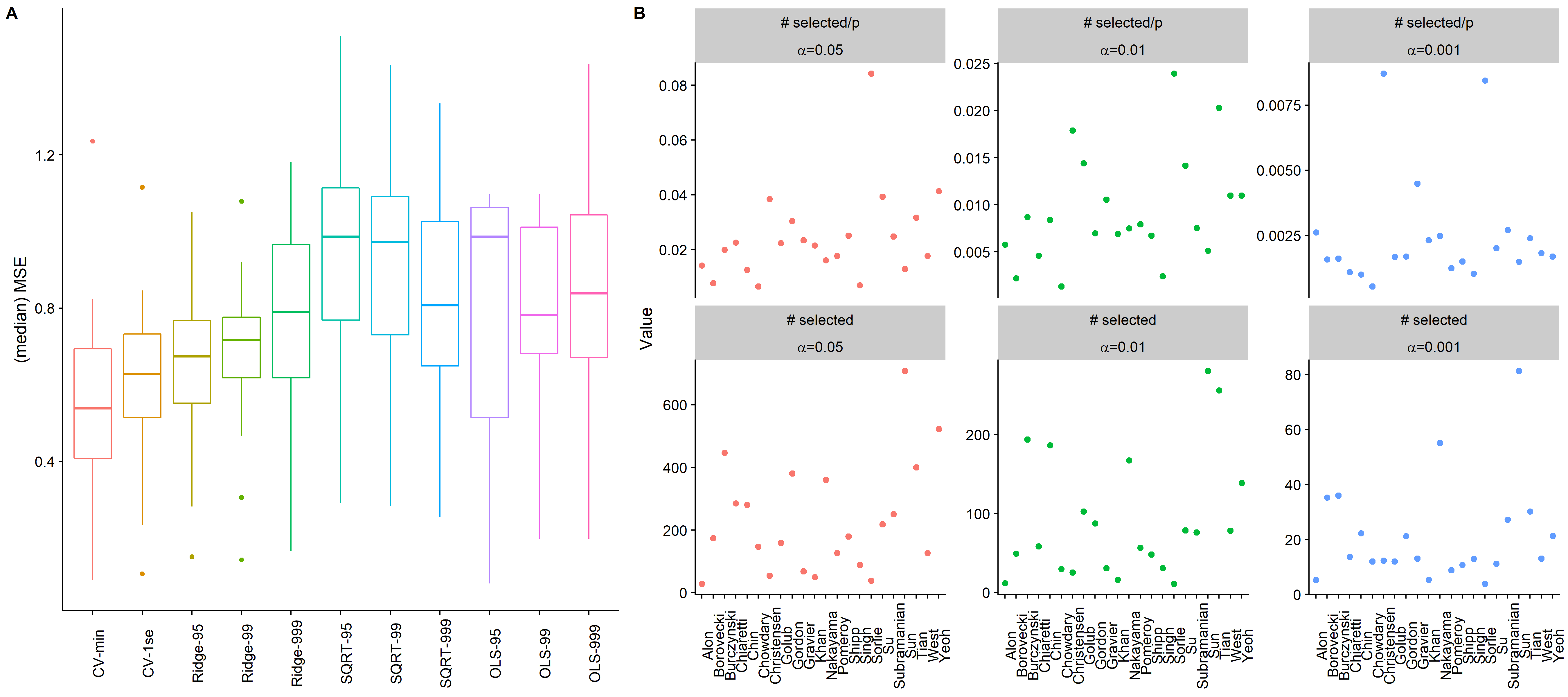
The prediction results on real-world datasets are revealing. They show that while the \(\sqrtl\), and theoretical approaches more generally, have elegant properties and can perform well for in simulation scenarios where the model is highly sparse (\(s < N\)), on real datasets the cross-validated Lasso appears to perform better. In some sense this is not surprising since CV specifically adapts itself to the bias-variance tradeoff found in any dataset.