Introduction

When comparing the performance of an individual or competing group of survival models, the most common choice of scoring metric is the concordance index (C-index). In the time-to-event setting, with \(N\) observations, the quality of a risk score can be determined by comparing how well the actual ordering of events occurs relative to the ranks of a model’s predicted risk score. There can be up to \(N(N-1)/2\) possible pairwise comparisons of rank-orderings for right-censored time-to-event data. For example if patient 1 died first, then ideally his risk score should be higher than patients 2, 3, … and \(N\), and if patient 2 died second his risk score should be higher than patients 3, 4, …, \(N\), and so on. Equation \eqref{eq:c_exact} formalizes this metric over a double sum.

Where \(\delta_i=1\) indicates that the patient has experienced the event, \(Y_j(t_i)\) is whether patient \(j\) has a recorded time greater than patient \(i\), \(\eta_i\) is the risk score of patient \(i\), \(I[\cdot]\) is the indicator function, and \(D\) is the cardinality of the set of all possible pairwise comparisons. Notice that the outer loop is zero if \(\delta_i=1\); this ensures that if \(T_i\) is right-censored (i.e. a patient lived for at least \(T_i\) units of time) they do not contribute to the final score.

Models that are commonly used in survival analysis (the Cox-PH, Random Survival Forest, CoxBoost, Accelerating Failure Time, etc) do not directly minimize a linear (or non-linear) set of features with respect to the C-index. In the case of the partial likelihood (associated with any of the “Cox” models) a sort-of-convex relaxation is used (it also includes a double sum) but more resembles a Softmax function. The goal of this post will be to show how to construct a convex loss function that directly lower-bounds the actual concordance index with the use of the log-sigmoid function. Other smooth functions could also be conceivably used. Readers are encouraged to see this excellent paper for a further discussion of the log-sigmoid lower bound.

Function for the concordance index

It is easy to write a wrapper to calculate the concordance index. This will be able to emulate the survConcordance() function from the survival package.

# Function for the i'th concordance
cindex_i <- function(So,eta,i) {
  tt_i <- So[i,1]
  dd_i <- So[i,2]
  idx.k <- which(So[,1] > tt_i)
  conc <- sum(eta[i] > eta[idx.k]  )
  disc <- sum(eta[i] < eta[idx.k]  )
  return(c(conc,disc))
}
 
 
# Wrapper for total concordance
cindex <- function(So,eta) {
  conc.disc <- c(0,0)
  for (i in which(So[,2] == 1)) {
    conc.disc <- conc.disc + cindex_i(So,eta,i)
  }
  names(conc.disc) <- c('concordant','discordant')
  return(conc.disc)
}

Using the veteran dataset as an example.

library(survival)
 
So <- with(veteran,Surv(time,status==1))
X <- model.matrix(~factor(trt)+karno+diagtime+age+factor(prior),data=veteran)[,-1]
eta <- predict(coxph(So ~ X))
 
Som <- as.matrix(So)
Som[,1] <- Som[,1] + (1-Som[,2])*min(Som[,1])/2
 
survConcordance.fit(So, eta)[1:2]

## concordant discordant 
##       6286       2518

cindex(Som, eta)

## concordant discordant 
##       6286       2518

Notice that a small amount of time is added to patients who were censored. This ensures that they will be measured as having lived longer than someone who experienced the event at the exact same time. This and other issues around handling ties in the concordance index are ignored in this post.

Convex relaxation of the C-index

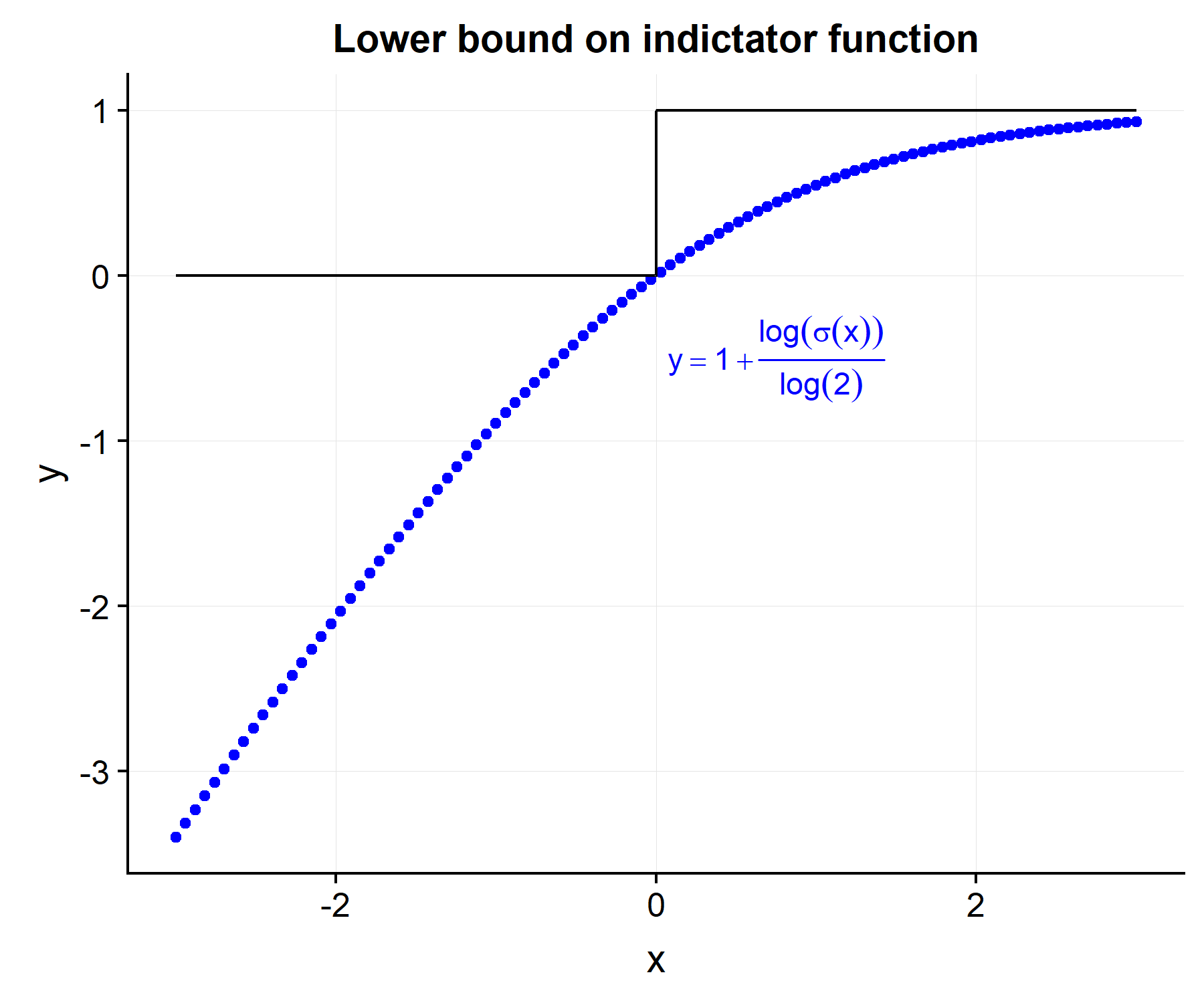
Because the C-index is sum of indicator functions, which are discrete, its optimizing problem is NP hard. By using a smooth and differentiable function which provides a lower bound on the indicator function, we will then have a convex optimization problem. Intuitively, a sigmoid-type function feels appropriate since its output is between zero and one. However it is not convex by itself. If we take a log-transform of the sigmoid function, then we have a concave function (and hence its negative is convex).

By doing some quick math it is easy to see that \(I(x>0) \leq [1+ \log(\sigma(x))/\log(2)]\) and hence \(C(\etab) \geq \tilde{C}(\etab)\).

However the derivative of \eqref{eq:c_approx}, unlike \eqref{eq:c_exact} can be taken with respect to the \(i^{th}\) risk score.

I drop any constants from \eqref{eq:c_approx}, as these can be ignored during optimization. When \(\eta_i = \xbi^T\betab\), the gradient becomes (via the chain-rule):

It is worth pausing to think about the terms inside the partial derivative in equation \eqref{eq:c_deriv}. The component in (a) encourages the risk score to be higher in patient \(i\) relative to all other patients who died after them i.e. the set \(k: Y_k(t_i)=1\), assuming that patient \(i\) is not censored. Countering this tendency is the term (b) which accounts for the fact that raising the \(i^{th}\) risk score decreases the distance between patient \(i\) and all the other people who died before her. It is also interesting to compare this “residual” [(a) - (b)] to the martingale residual seen in the Cox model as a comparison.

While the convex relaxation of the C-index and the Cox model both have double sums and both encourage a higher risk score for patients who experienced the event before other patients, the former is purely a linear combination of terms. The next code blocks calculate the convex loss function and its derivative.

\(\tilde{C}(\etab)\) from \eqref{eq:c_approx}:

sigmoid <- function(x) { 1/(1+exp(-x)) }
 
l_eta_i <- function(So,eta,i) {
  tt_i <- So[i,1]
  dd_i <- So[i,2]
  idx.k.i <- which(So[,1] > tt_i)
  loss.i <- sum(1 + log( sigmoid(eta[i] - eta[idx.k.i]) )/log(2) )
  return(loss.i)
}
 
l_eta <- function(So, eta) {
  loss <- 0
  for (i in which(So[,2] == 1)) {
    loss <- loss + l_eta_i(So,eta,i)
  }
  return(-loss / nrow(So)^2)
}

\(\partial \tilde{C}(\betab) / \partial \betab\) from \eqref{eq:c_deriv}:

sigmoid2 <- function(x) { 1/(1+exp(x)) }
 
dl_eta_i <- function(eta,So,i) {
  tt_i <- So[i,1]
  dd_i <- So[i,2]
  idx.k <- which(So[,1] > tt_i)
  idx.j <- which(tt_i > So[,1] & So[,2]==1) 
  res.i <- dd_i*sum(sigmoid2(eta[i] - eta[idx.k])) - sum(sigmoid2(eta[idx.j] - eta[i]))
  return(res.i)
}
 
dl_eta <- function(X,eta,So) {
  grad <- rep(0, ncol(X))
  for (i in seq_along(eta)) {
    grad <- grad + X[i,] * dl_eta_i(eta, So, i)
  }
  grad <- -1 * grad / nrow(X)^2
  return(grad)
}

Simulation examples

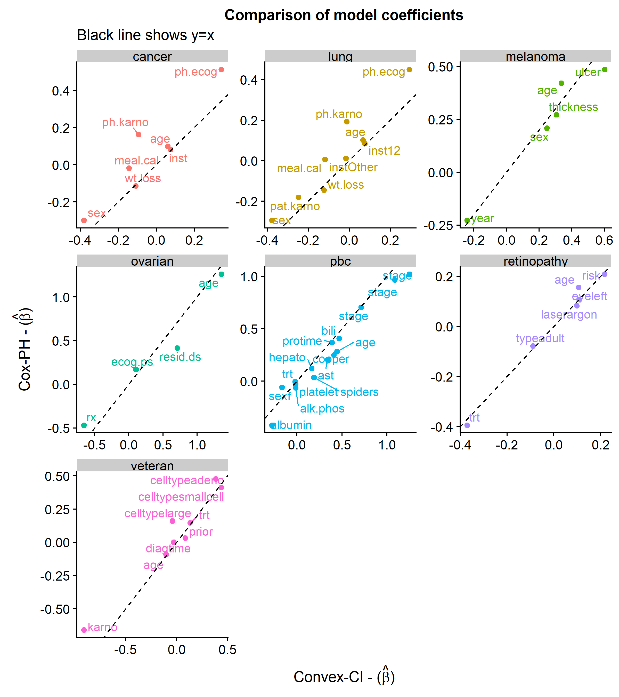
How much better does this convex approximation perform on the actual concordance index compared to the Cox model? Based on simulations using seven datasets from the survival package: cancer, lung, melanoma, ovarian, pbc, retinopathy, and veteran, there is a marginal improvement in test set accuracy for four of them.

The first plot below shows the similarities in the coefficients between the two approaches.

The next plot shows a comparison of the distribution of C-index scores across 250 simulations using an 80/20 train/test split.

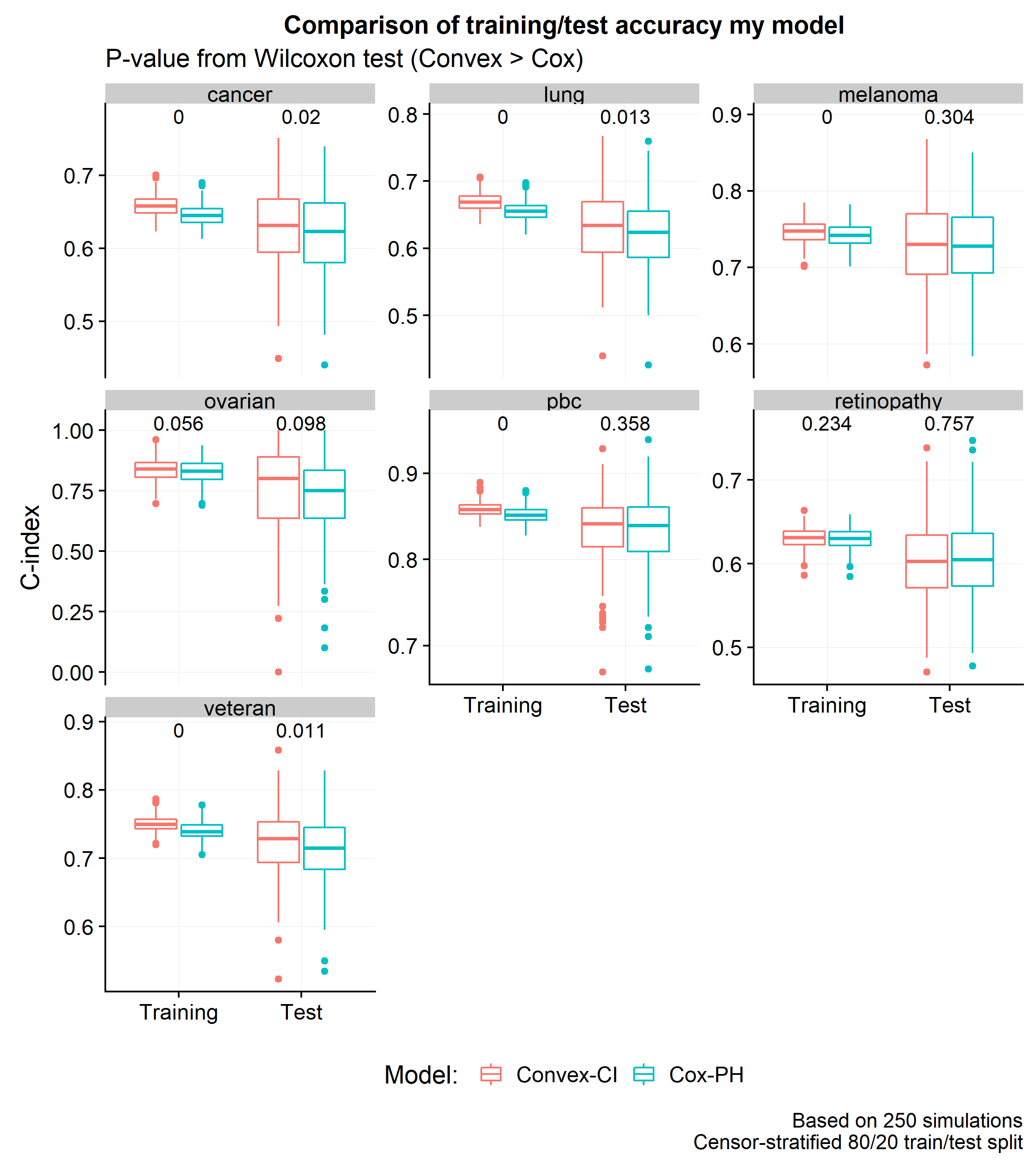
It is interesting that by changing the loss function, one can boost the training and test C-index scores by around 0.8% and 0.6% (respectively). However, the most important result of this post is that the convex approximation of the C-index does no worse than the partial likelihood loss and has one crucial computational advantage: the gradient is a sum of linear terms (unlike the partial likelihood with has a fraction). Stochastic gradient descent methods will allow for these models to easily scale up to massive datasets – a discussion which will be explored in a subsequent post.