Summary

This post reviews the fragility index, a statistical technique proposed by Walsh et. al (2014) to provide an intuitive measure of the robustness of study findings. I show that the distribution of the fragility index can be approximated by a truncated Gaussian whose expectation is directly related to the power of the test (see equation \eqref{eq:fi_power}). This evidence will hopefully clarify the debate around what statistical quantity the fragility index actually represents. Even though the fragility index can provide a conservative estimate of the power of a study, on average, it is a very noisy indicator. In the final sections of this post I provide arguments both in favour and against the fragility index. To replicate all figures in this post, see this script.

(1) Background

Most published studies have exaggerated effect sizes. There are two main reasons for this. First, scientific research tends to be under-powered. This means that studies do not have enough samples to be able to detect small effects. Second, academic journals incentivize researchers to publish “novel” findings that are statistically significant. In other words, researchers are encouraged to try different variations of statistical tests until something “interesting” is found.[¹]

As a reminder, the power of a statistical test defines the probability that an effect will be detected when it exists. Power is proportional to the sample size for consistent tests because more samples leads to tighter inference around some effect size.

Most researchers are aware of the idea of statistical power, but a much smaller share understand that it is directly related to effect size bias. Conditional on statistical significance, all measured effects are biased upwards because there is a minimum effect size needed for a test to be considered statistically significant.[²] Evidence that most fields of science are under-powered in practice are numerous (see here or here). Many disciplines do not even require studies to make power justifications before research begins.[³]

Some researchers have attempted to justify the sample sizes of their studies by doing post-hoc (after-the-fact) power calculations using the estimated effect size as the basis for their estimates. This approach is problematic for three reasons. First, post-hoc power using the measured effect size as the assumed effect size is mathematically redundant since it has a one-to-one mapping with the conventionally calculated p-value. Second, this type of post-hoc power will always show high power for statistically significant results, and low power for statistically insignificant results (this helpful post explains why).[⁴] Lastly, in underpowered designs, the estimated effect will be noisy, making post-hoc estimates of power equally as noisy!

The fragility index (FI) is relatively new statistical technique that uses an intuitive approach to quantify post-hoc robustness in studies with a binary outcomes framework with two groups. Qualitatively, the FI states how many patients in the treatment group would need to have their status swapped from event to non-event in order for the trial to be statistically insignificant.[⁵] In the original Walsh paper, the FI was calculated for RCTs published in high impact medical journals. They found median FI of 8, and a 25% quantile of 3.

Since the original Walsh paper, the FI has been applied hundreds of times to other areas of medical literature.[⁶] Most branches of medical literature show a median FI that is in the single digits. While the FI has its drawbacks (discussed below), this new approach appears to have captured the statistical imagination of researchers in a way that power calculations have not. While being told that a study has 20% power should cause immediate alarm, it apparently does not cause the same level of concern as finding out an important cancer drug RCT was two coding errors away from being deemed ineffective.

The rest of this post is organized as follows: section (2) provides an explicit relationship between the fragility index and the power of the test, section (3) provides an algorithm to calculate the FI using python code, section (4) reviews the criticisms against FI, and section (5) concludes.

(2) Binomial proportion fragility index (BPFI)

This section examines the distribution of the FI when the test statistic is the normal-approximation of a difference in a binomial proportion; hereafter referred to as the binomial proportion fragility index (BPFI). While Fisher’s exact test is normally used for estimating the FI, the BPFI is easier to study because it has an analytic solution. Two other simplifications will be used in this section for ease of analysis. First, the sample sizes will be the same between groups, and second, a one-sided hypothesis test will be used. Even though the BPFI may not be standard, it is a consistent statistic that is asymptotically normal and is just as valid as using other asymptotic statistics like a chi-squared test.

The notation used will be as follows: the statistic is the difference in proportions, \(d\), whose asymptotic distribution is a function of the number of samples and the respective binary probabilities (\(\pi_1, \pi_2\)):

Assume that \(n_1 = n_2 = n\) and the null-hypothesis is \(\pi_2 \leq \pi_1\). We want to test whether group 1 has a larger event rate than group 2.

Notice that when calculating the variance of the test statistic when the null is false, the event rate pools the events across groups. For a given type-1 error rate target (\(\alpha\)), and corresponding rejection threshold, the power of the test when the null is false can be calculated:

The formula \eqref{eq:power} shows that increasing \(\pi_d\), \(n\), or \(\alpha\) all increase the power. Figure 1 below shows that the formula to estimate power is a close approximation for reasonable sample sizes.

Given that the null has been rejected, the roots of the equation can be solved to find the exact point of statistical insignificance using the quadratic formula.

While equation \eqref{eq:fi1} is exact, the FI can be approximated by assuming the variance is constant:

As Figure 2 shows below, \eqref{eq:fi2} is very close to the \eqref{eq:fi1} for reasonably sized draws (\(n=200\)).

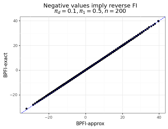
Next, we can show that the approximation of the BPFI from \eqref{eq:fi2} is equivalent to a truncated Gaussian when conditioning on statistical significance.

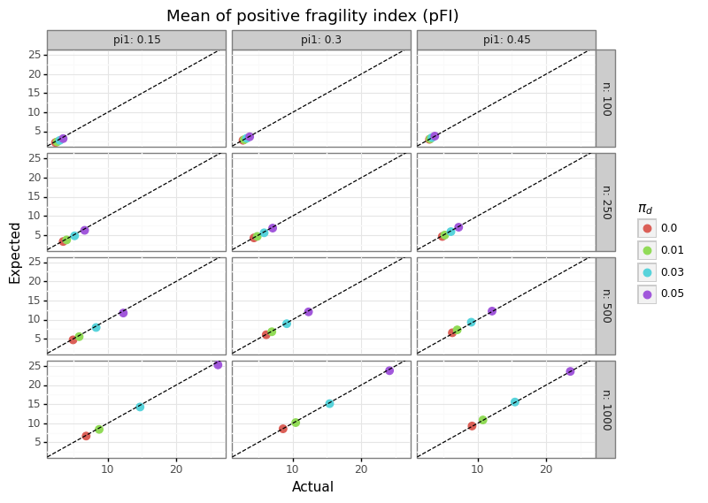
\(\begin{align*} \text{pFI}_a &= \text{FI}_a \hspace{2mm} \big| \hspace{2mm} \text{FI}_a > 0 \hspace{2mm} \longleftrightarrow \\ \text{FI}_a &\sim N \big( n\pi_d - t_\alpha\sqrt{2n \pi_0(1-\pi_0)}, n[\pi_1(1-\pi_1) + \pi_2(1-\pi_2)] \big) \\ E[\text{pFI}_a] &= n\pi_d - t_\alpha\sqrt{2n \pi_0(1-\pi_0)} + \sqrt{n[\pi_1(1-\pi_1) + \pi_2(1-\pi_2)]} \frac{\phi(-E[\text{FI}_a]/\text{Var}[\text{FI}_a]^{0.5})}{\Phi(E[\text{FI}_a/\text{Var}[\text{FI}_a]^{0.5}])} \end{align*}\)

Figure 3 below shows that the truncated Gaussian approximation does a good job at estimating the actual mean of the BPFI.

If the positive BPFI is divided by root-n and the variance under the alternative (a constant) we obtain a monotonic transformation of the fragility index:

Where \(\beta\) is the type-II error rate (i.e. one minus power). Figure 4 below shows power estimates obtained by solving equation \eqref{eq:fi_power} for \(1-\beta\) for the statistically significant results.

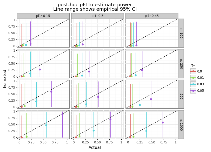
While the median power estimate is a conservative estimate to the actual value, the empirical variation is tremendous. Why is there so much variation? The answer is simple: the distribution of FIs is similar for different effect sizes as Figure 5 shows below.

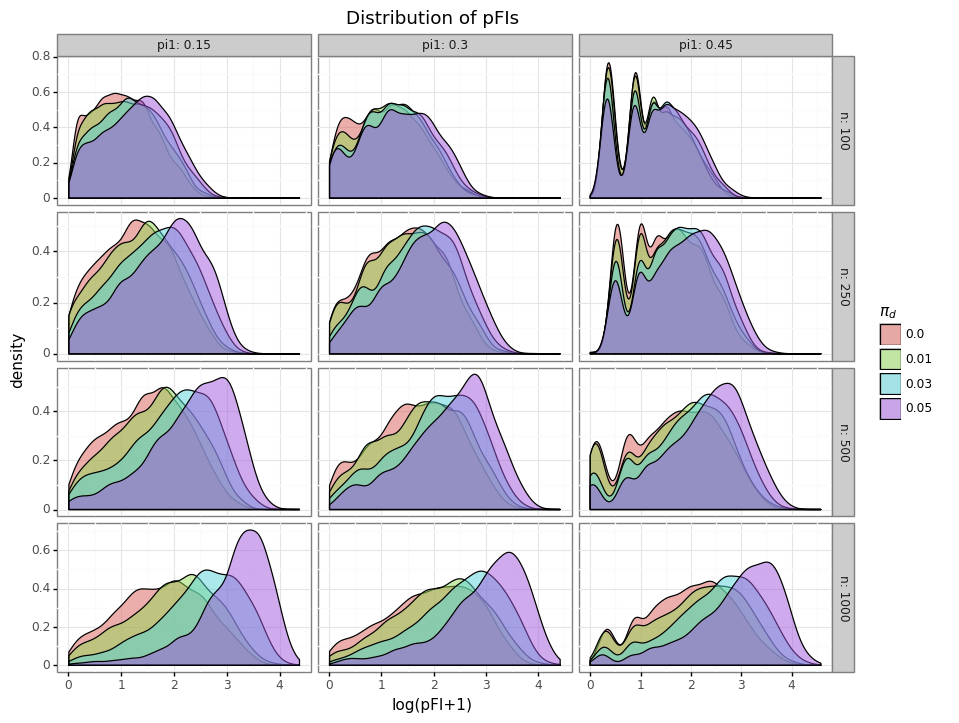
Even though a test may have a power of 75%, it will have a similar distribution of FIs to another test that has only 10% power. This naturally means that there will be significant uncertainty around the true power for any measured FI.

(3) Calculating the fragility index

Consider the classical statistical scenario of a 2x2 table of outcomes, corresponding to two different groups with a binary outcome recorded for each group. For example, a randomized control trial (RCT) for a medical intervention usually corresponds to this scenario where the two groups are the (randomized) treatment and control group and the study records some event indicator associated with a health outcome.

Suppose in this trial that the event rate is greater in treatment than the control group, and that this positive difference is statistically significant. If a patient who was recorded as having an event in the treatment group has their entry “swapped” to a non-event, then the proportions between the groups will narrow, and the result will become less statistically significant by definition. For any test statistic, the FI can be defined as follows:

Where \(n_i=n_{iA}+n_{iB}\) is the total number of samples for group \(i\), and there are \(n_{iA}\) events. The code below provides the wrapper function FI_func needed to calculate the fragility index using the methodology as originally proposed. The sample sizes for both groups are fixed, with the event rate being modified for only group 1. The algorithm works by iteratively flipping one patient from event to non-event (or vice-versa) until there is a change in statistical significance. While a naive approach is simply to initialize the contingency table with the original data, a significant speed-up can be accrued by estimating the FI with the BPFI as discussed in section 2. Conditional on any starting point, the algorithm converges by applying the following rule:

1. Flip event to non-event in group 1 if event rate is larger in group 1 and current result is statistically significant
2. Flip non-event to event in group 1 if event rate is larger in group 1 and current result is statistically insignificant
3. Flip non-event to event in group 1 if event rate is smaller in group 1 and current result is statistically significant
4. Flip event to non-event in group 1 if event rate is smaller in group 1 and current result is statistically insignificant

Why would the direction be changed if the result is insignificant? This occurs when the BPFI initialization has overshot the estimate. For example, imagine the baseline event rate is 50/1000 in group 1 and 100/1000 in group 2, and the BPFI estimates that insignificance occurs at 77/1000 for group 1. When we apply the Fisher’s exact test, we find that insignificance actually occurs at 75/1000, and to discover this we need to subtract off events from group 1 until the significance sign changes. In contrast, if the BPFI estimates that insignificance occurs at 70/1000, then when we run Fisher’s exact test, we’ll find that the results are still significant and will need to add patients to the event category until the significance sign changes.

As a final note, there are two other ways to generate variation in the estimate of the FI for a given data point:

1. Which group is considered “fixed”
2. Which statistical test is used

To generate the first type of variation, the values of n1A/n1 and n2A/n2 can simply be exchanged. Any function which takes in an 2x2 table and returns a p-value can be used for the second. I have included functions for Fisher’s exact and the Chi-squared test.

import numpy as np
import scipy.stats as stats

"""
INPUT
n1A:      Number of patients in group1 with primary outcome
n1:       Total number of patients in group1
n2A:      Number of patients in group2 with primray outcome
n2:       Total of patients in group2
stat:     Function that takes a contingency tables and return a p-value
n1B:      Can be specified is n1 is None
n2B:      Can be specified is n2 is None
*args:    Will be passed into statsfun

OUTPUT
FI:       The fragility index
ineq:     Whether group1 had a proportion less than or greater than group2
pv_bl:    The baseline p-value from the Fisher exact test
pv_FI:    The infimum of non-signficant p-values
"""
def FI_func(n1A, n1, n2A, n2, stat, n1B=None, n2B=None, alpha=0.05, verbose=False, *args):
  assert callable(stat), 'stat should be a function'
  if (n1B is None) or (n2B is None):
    assert (n1 is not None) and (n2 is not None)
    n1B = n1 - n1A
    n2B = n2 - n2A
  else:
    assert (n1B is not None) and (n2B is not None)
    n1 = n1A + n1B
    n2 = n2A + n2B
  lst_int = [n1A, n1, n2A, n2, n1B, n2B]
  assert all([isinstance(i,int) for i in lst_int])
  assert (n1B >= 0) & (n2B >= 0)
  # Calculate the baseline p-value
  tbl_bl = [[n1A, n1B], [n2A, n2B]]
  pval_bl = stat(tbl_bl, *args)
  # Initialize FI and p-value
  di_ret = {'FI':0, 'pv_bl':pval_bl, 'pv_FI':pval_bl, 'tbl_bl':tbl_bl, 'tbl_FI':tbl_bl}
  # Calculate inital FI with binomial proportion
  dir_hypo = int(np.where(n1A/n1 > n2A/n2,+1,-1))  # Hypothesis direction
  pi0 = (n1A+n2A)/(n1+n2)
  se_null = np.sqrt( pi0*(1-pi0)*(n1+n2)/(n1*n2) )
  t_a = stats.norm.ppf(1-alpha/2)
  bpfi = n1*(n2A/n2+dir_hypo*t_a*se_null)
  init_fi = int(np.floor(max(n1A - bpfi, bpfi - n1A)))
  if pval_bl < alpha:
    FI, pval, tbl_FI = find_FI(n1A, n1B, n2A, n2B, stat, alpha, init_fi, verbose, *args)
  else:
    FI, pval = np.nan, np.nan
    tbl_FI = tbl_bl
  # Update dictionary
  di_ret['FI'] = FI
  di_ret['pv_FI'] = pval
  di_ret['tbl_FI'] = tbl_FI
  di_ret
  return di_ret

# Back end function to perform the for-loop
def find_FI(n1A, n1B, n2A, n2B, stat, alpha, init, verbose=False, *args):
  # init=init_fi
  assert isinstance(init, int), 'init is not an int'
  assert init > 0, 'Initial FI guess is less than zero'
  n1a, n1b, n2a, n2b = n1A, n1B, n2A, n2B
  n1, n2 = n1A + n1B, n2A + n2B
  prop_bl = int(np.where(n1a/n1 > n2a/n2,-1,+1))

  # (i) Initial guess
  n1a = n1a + prop_bl*init
  n1b = n1 - n1a
  tbl_int = [[n1a, n1b], [n2a, n2b]]
  pval_init = stat(tbl_int, *args)
  
  # (ii) If continues to be significant, keep direction, otherwise flip
  dir_prop = int(np.where(n1a/n1 > n2a/n2,-1,+1))
  dir_sig = int(np.where(pval_init<alpha, +1, -1))
  dir_fi = dir_prop * dir_sig
  
  # (iii) Loop until significance changes
  dsig = True
  jj = 0
  while dsig:
    jj += 1
    n1a += +1*dir_fi
    n1b += -1*dir_fi
    assert n1a + n1b == n1
    tbl_dsig = [[n1a, n1b], [n2a, n2b]]
    pval_dsig = stat(tbl_dsig, *args)
    dsig = (pval_dsig < alpha) == (pval_init < alpha)
  vprint('Took %i iterations to find FI' % jj, verbose)
  if dir_sig == -1:  # If we're going opposite direction, need to add one on
    n1a += -1*dir_fi
    n1b += +1*dir_fi
    tbl_dsig = [[n1a, n1b], [n2a, n2b]]
    pval_dsig = stat(tbl_dsig, *args)

  # (iv) Calculate FI
  FI = np.abs(n1a-n1A)
  return FI, pval_dsig, tbl_dsig

# Wrappers for different p-value approaches
def pval_fisher(tbl, *args):
  return stats.fisher_exact(tbl,*args)[1]

def pval_chi2(tbl, *args):
  tbl = np.array(tbl)
  if np.all(tbl[:,0] == 0):
    pval = np.nan
  else:
    pval = stats.chi2_contingency(tbl,*args)[1]
  return pval

def vprint(stmt, bool):
  if bool:
    print(stmt)

FI_func(n1A=50, n1=1000, n2A=100, n2=1000, stat=pval_fisher, alpha=0.05)

{'FI': 25,
 'pv_bl': 2.74749805216798e-05,
 'pv_FI': 0.057276449223784075,
 'tbl_bl': [[50, 950], [100, 900]],
 'tbl_FI': [[75, 925], [100, 900]]}

As the output above shows, the FI_func returns the FI and corresponding table at the value of insignificance. If the groups are flipped, one can show the FI for group 2:

FI_func(n1A=100, n1=1000, n2A=50, n2=1000, stat=pval_fisher, alpha=0.05)

{'FI': 29,
 'pv_bl': 2.74749805216798e-05,
 'pv_FI': 0.06028540160669414,
 'tbl_bl': [[100, 900], [50, 950]],
 'tbl_FI': [[71, 929], [50, 950]]}

Notice that the FI is not symmetric. When the baseline results are insignificant, the function will return a np.nan.

FI_func(n1A=71, n1=1000, n2A=50, n2=1000, stat=pval_fisher, alpha=0.05)

{'FI': nan,
 'pv_bl': 0.06028540160669414,
 'pv_FI': nan,
 'tbl_bl': [[71, 929], [50, 950]],
 'tbl_FI': [[71, 929], [50, 950]]}

(4) Criticisms of the FI

There are two main criticisms levelled against the FI. First, it does not do what it claims to do on a technical level, and second that it encourages null hypothesis significance testing (NHST). The first argument can be seen in Potter (2019), which shows that the FI is not comparable between studies because it does not quantify how “fragile” the results of a study actually are. Specifically, the paper shows that the FI does not provide evidence as to how likely the null hypothesis is relative to the alternative (i.e. that there is some effect). If there are two identically powered trials with differences in sample sizes, then it must be the case that the trial with a smaller sample size has a larger effect size. By looking at the Bayes factor, Potter shows that for any choice of prior, a smaller trial with a larger effect size is more indicative of an effect existing than a larger trial with a smaller effect size for a given power.

Therefore, if the probability model is correct (as in the coin toss example), the small trial provides more evidence for the alternative hypothesis than the large one. It should not be penalized for using fewer events to demonstrate significance. When the probability model holds, the FI incorrectly concludes that the larger trial provides stronger evidence. (Potter 2019)

For example, a study with 100 patients might have a p-value of 1e-6 and a FI of 5, whereas a study with 1000 patients with a p-value of 0.03 might have a FI of 10. In other words, the FI tends to penalize studies for being small, rather than studies that have a weak signal. Furthermore, the fragility index will often come to the opposite conclusion of a Bayes factor analysis.

Altogether, the FI creates more confusion than it resolves and does not promote statistical thinking. We recommend against its use. Instead, sensitivity analyses are recommended to quantify and communicate robustness of trial results. (Potter 2019)

A second criticism of the FI is that it encourages thinking in the framework of NHST and its associated problems. As Perry Wilson articulates, the FI further entrenches dichotomous thinking when doing statistical inference. For example, if a coin is flipped 100 times, and 60 of them are heads, using a 5% p-value cut-off, the null of an unbiased coin (p-value=0.045) will be rejected. But such a result has a FI of one, since 59 heads would have a p-value of 0.07. However, both results are “unlikely” under the null, so it seems strange to conclude the the initial finding should be discredited because of a FI of one.

(5) Conclusion

While others papers have shown correlations between the empirical FI and post-hoc power (see here, here, or here), my work is the first (I believe) to show an explicit analytic relationship between power and the expected value of the FI, when using a binomial proportions test.

The Potter paper is correct: the FI does not provide insight into the posterior probabilities between studies. Rather, it provides a noisy and conservative estimate of the power. As section (2) showed, unlike other types of post-hoc power analyses, the FI is able to show low power, even for statistically significant results, because using the first moment of the truncated Gaussian explicitly conditions on this significance filter. However, inverting this formula to estimate the power leads to results that are too noisy in practice to use with any confidence (see Figure 4).

I agree with the criticisms of the FI highlighted in section (4), but the method can still be defended on several grounds. First, the FI can be made more comparable between studies by normalizing the number of samples (known as the fragility quotient (FQ)). Second, smaller studies should be penalized in a frequentist paradigm, not because their alternative hypothesis is less likely to be true (which is what the Bayes factor tells us), but rather because the point estimate of the statistic conditional on significance is going to be exaggerated. Lastly, even though the FI does encourage dichotomous thinking, that is a problem of the NHST and not the FI per se.

To expand on the analogy of the biased coin, if the world’s scientists went around flipping every coin they found lying on the sidewalk 100 times and then submitting their “findings” to journals every time they got 60 or more heads, then the world would appear to be festooned with biased coins. The bigger problem is that it is a silly endeavour to look around the world for biased coins. And even though there may be many coins with a slight bias (say 50.1% chance of heads) the observed (i.e. published) biases would be at least 10% more extreme than what should be reported. This highlights the bigger problem of scientific research and the file drawer issue.

I think the best argument in favour of the FI is that it encourages researchers to carry out studies with larger sample sizes. The real reason this should be done is to increase power, but if researchers are motivated because they don’t want a small FI, then so be it. Until now, researchers have developed all sorts of mental ju-jitsu techniques to defend their under-powered studies. Such techniques include the “whatever doesn’t kill my p-value makes it stronger” argument.[⁷] Not to pick on Justin Wolfers, but here is one example of such a sentiment:

You are suggesting both GDP and happiness are terribly mismeasured. And the worse the measurement is the more that biases the estimated correlation towards zero. So it’s amazing that the estimated correlation is as high as 0.8, given that I’m finding that’s a correlation between two noisy measures.

Noise makes my claim stronger! Making such a statement against a more intuitive measure like the FI would be harder. As the authors of the original Welsh paper put it:

The Fragility Index has the merit that it is very simple and may help integrate concerns over smaller samples sizes and smaller numbers of events that are not intuitive. We conclude that the significant results of many RCTs hinge on very few events. Reporting the number of events required to make a statistically significant result nonsignificant (ie, the Fragility Index) in RCTs may help readers make more informed decisions about the confidence warranted by RCT results.

Footnotes