Background

Validating machine learning (ML) models in a prospective setting is a necessary, but not a sufficient condition, for demonstrating the possibility algorithmic utility. Most models designed on research datasets will fail to translate in a real-word setting. This problem is referred to as the “AI chasm”.[¹] There are numerous reasons why this chasm exists. Retrospective studies have numerous “researchers degrees of freedom” which can introduce an optimism bias in model performance. Extracting data retrospectively ignores many technical challenges that occur in a real-time setting. For example, most data fields have vintages, meaning their value will differ depending on when they are queried. This is because data often undergoes revisions or adjustments during its collection. From an ethical perspective, a prospective trial of an ML model is a necessary condition to justify equipoise.

I have already written two previous posts about how to prepare and evaluate a binary classifier and regression model for a statistical trial. In this post I will again return to the problem of validating a binary classifier. However, this analysis will consider how to test two performance measures simultaneously: sensitivity (the true positive rate) and specificity (the true negative rate). In the previous formulation I wrote about, calibrating the binary classifier was a three stage process:

1. Using the bootstrap to approximate the distribution of operating thresholds that achieves a given performance measure.
2. Choosing a conservative operating threshold that achieves that performance measure at least \((1-\alpha)\)% of the time.
3. Carrying out a power estimate assuming that the performance measure will be met by the conservative operating threshold.

For example, suppose the goal is to have a binary classifier achieve 90% sensitivity. First, the positive scores would be bootstrapped 1000 times. For each bootstrapped sample of data, a threshold would be found that obtains 90% sensitivity (i.e. the 10% quantile of bootstrapped data). Second, the 5% quantile of those 1000 thresholds would be chosen. This 5% quantile approximates the lower-bound point of a one-sided 95% confidence interval (CI). This procedure will, (approximately) 95% of the time, select a threshold that obtains at least 90% sensitivity.[²] Third, the power of the statistical trial would be assessed as a function of the null hypothesis and sample size, assuming the classifier actually achieves 90% sensitivity. Because the randomness of the operating threshold is bounded, the power analysis can be assumed to be exact (while in reality it will be conservative).[³]

If the goal of a statistical trial is to show that the model has certain level of both sensitivity and specificity, then the picking a conservative operating threshold is impossible. Any attempts to pick a lower-bound estimate of the threshold to increase sensitivity will necessarily decrease the likelihood of meeting a specificity target, and vice versa. This post will outline an approach that picks an empirical operating threshold, and then provide an uncertainty estimate around the subsequent power analysis. In other words, the power of the trial will itself become a random variable. The sample size and null hypothesis margin will still impact the power, of course, but there will now be uncertainty around the actual power of the trial.

The rest of the post is structured as follows. Section (2) explains the ROC curve and how to select an operating threshold that trades off between sensitivity and specificity. Section (3) describes the inherent uncertainty in the power analysis when an empirical threshold is chosen on a finite sample of data. Section (4) provides simulation evidence as to the accuracy of the proposed methodology. Section (5) concludes.

The code used to produce these figures and analysis can be found here.

(1) Notation and assumptions

Assume there is an existing ML algorithm with a learned a set of parameters \(\theta\) that maps a \(p\)-dimensional input \(x\) to a single real-valued number: \(g_\theta(x): \mathbb{R}^p \to \mathbb{R}\). The output of this function is referred to as a score \(g_\theta(x)=s\). For a binary outcomes model, the target label (\(y\)) is either a zero (negative class) or a one (positive class), \(y \in \{0, 1\}\). A higher score indicates the label is more likely to be a 1. To do actual classification, an operating threshold (\(t\)) must be selected so that the scores are binarized: \(\psi_t(g): \mathbb{R} \to \{0, 1\}\). We denote the predicted label of the model by \(z\), \(\psi_t(s(x)) = I(g_\theta(x)\geq t) = I(s \geq t) = z\). Subscripts will, in general, be used to indicate a conditional distribution or class-specific parameter. Thus, \(n_1\) and \(n_0\) indicate the number of positive and negative samples, respectively.

Unless stated otherwise, the data generating process of the scores coming from the model will have a conditionally Gaussian distribution: \(s_1=s|y=1\sim N(\mu,1)\) and \(s_0=s|y=0\sim N(0,1)\). None of the statistical procedures described in this post rely on the scores being Gaussian. This simplifying assumption is done so that simulation results can compared to an oracle value. Cumulative distribution functions (CDFs) and probability density functions (PDFs) will be represented by \(F\) and \(f\), respectively. In the case of the standard normal, \(\Phi\) and \(\phi\) will be used instead. \(F^{-1}(k)\) refers to the (100\(k\))% quantile of a distribution.

Statistical estimators will often be compared to a “ground truth”, “long-run”, “expected”, or “oracle” value. When these terms are used, they refer to the value that would be picked if the true underlying data distribution were known, and will often be denoted by the star superscript. For example, if \(m\sim N(0,1)\) then the oracle choice for \(t\) for \(P(m > t) = 0.5\) would be \(t^{*}=0\).

A hat indicates either an estimator or a realization of a random variable. For example, \(\hat\mu_1 = n_1^{-1} \sum_{i=1}^{n_1}s_{i1}\) is the estimator for the mean of the positive scores. A realization of the score is indicated by a draw of the feature space: \(\hat{s} = g_\theta(\hat{x})\). For the operating threshold, the subscript will indicate the target of the performance measure. For example, \(\hat t_{\gamma}\) would be the operating threshold that obtains (100\(\gamma\))% empirical sensitivity (or specificity), whilst \(t^{*}_\gamma\) would be the operating threshold that obtains (100\(\gamma\))% sensitivity (or specificity) in expectation.

Calibration of the operating threshold occurs on an unused test set that the model has not been trained on. The test set is a representative draw of the the true underlying data generating process. By assuming the test set to be representative, problems around dataset shift are ignored. The prospective statistical trial that occurs subsequently if referred to as the “trial set.”

(2) The Receiver operating characteristic

The receiver operating characteristic (ROC) curve is a graphical representation of the trade-off between sensitivity (the true positive rate (TPR)), and specificity (true negative rate (TNR)), for a binary classifier. Because the TNR is one less the false positive rate (FPR), it can also be thought of as the trade-off between true positives (TPs) and false positives (FPs). This trade-off exists because the scores from a model need to binarized at a specific operating threshold to do classification. Ceteris paribus, decreasing the operating threshold will increase the number of TPs because the number of predicted positives will increase. Similarly, increasing the operating threshold increases the number of true negatives (TNs) because the number of predicted negatives will increase.

\[\begin{align*} TPR(t) &= P(s_{1} \geq t) \\ FPR(t) &= P(s_{0} \geq t) \\ TNR(t) &= P(s_{0} < t) \\ FNR(t) &= P(s_{1} < t) \end{align*}\]

The only free parameter the ML classifier has after model training is to set the operating threshold. All subsequent statistical properties of this classifier and its corresponding TPR and FPR flow from this choice. When the scores follow the conditional Gaussian distribution discussed in Section (1), then the TPR and FPR can be expression as a function of the operating threshold in a Gaussian CDF.

\[\begin{align*} TPR(t) &= \Phi(\mu - t) \\ TNR(t) &= \Phi(t) \end{align*}\]

The oracle ROC curve is therefore a set of tuples across all thresholds in the support of the score distribution \eqref{eq:oracle_roc}.

\[\begin{align*} &\text{Oracle ROC curve} \\ \forall t \in \mathbb{R}&: \{TPR(t), 1-TNR(t) \} \\ \forall t \in \mathbb{R}&: \{\Phi(\mu - t), \Phi(-t) \} \tag{1}\label{eq:oracle_roc} \\ \end{align*}\]

The larger the degree of class separation in the scores (\(\mu\)), the less severe the trade-off will be for the TPR and the FPR. For example, if \(\mu=2\) and \(t=2\), the TPR would be \(\Phi(0)=50\%\), whilst the FPR would be \(\Phi(-2)\approx 2.2\%\). The empirical ROC curve is an approximation of the oracle ROC curve. This curve uses the class-specific empirical CDFs (eCDFs) to approximate this relationship.

\[\begin{align*} &\text{Empirical ROC curve} \\ \forall t \in \mathbb{R}&: \{\hat{TPR}(t), \hat{FPR}(t) \} \\ \forall t \in \mathbb{R}&: \{\hat{F}_1(-t), \hat{F}_0(-t) \} \tag{2}\label{eq:emp_roc} \\ \end{align*}\]

Because the eCDF is discrete (\(\hat{F}\)), the ROC curve is a step function. A common summary statistic of the ROC curve is the Area Under the ROC curve (AUROC). However, the AUROC can hide important information. Different scores distributions can have the same AUROC, whilst having a fundamentally different trade-off between the TPR and the FPR. Figure 1A below shows three different ROC curve for skew normal distributions that have the same expected AUROC. For scores with a left-skew (Figure 1B), a low FPR can obtained with a relative high TPR. This is desirable for situations where the model needs to have a high precision. When the scores are left skewed, the positive class density (\(f_1\)) is much larger on the right side of the tail than is the negative class density (\(f_0\)). In contrast, when the scores are right skewed, a high sensitivity can be obtained with a relatively low FPR. This is desirable when false negatives need to be avoided.[⁴] This happens because the left-sided tails are relatively shallow so that a low threshold captures almost all of the positive instances.

Figure 1: Three example ROC curves

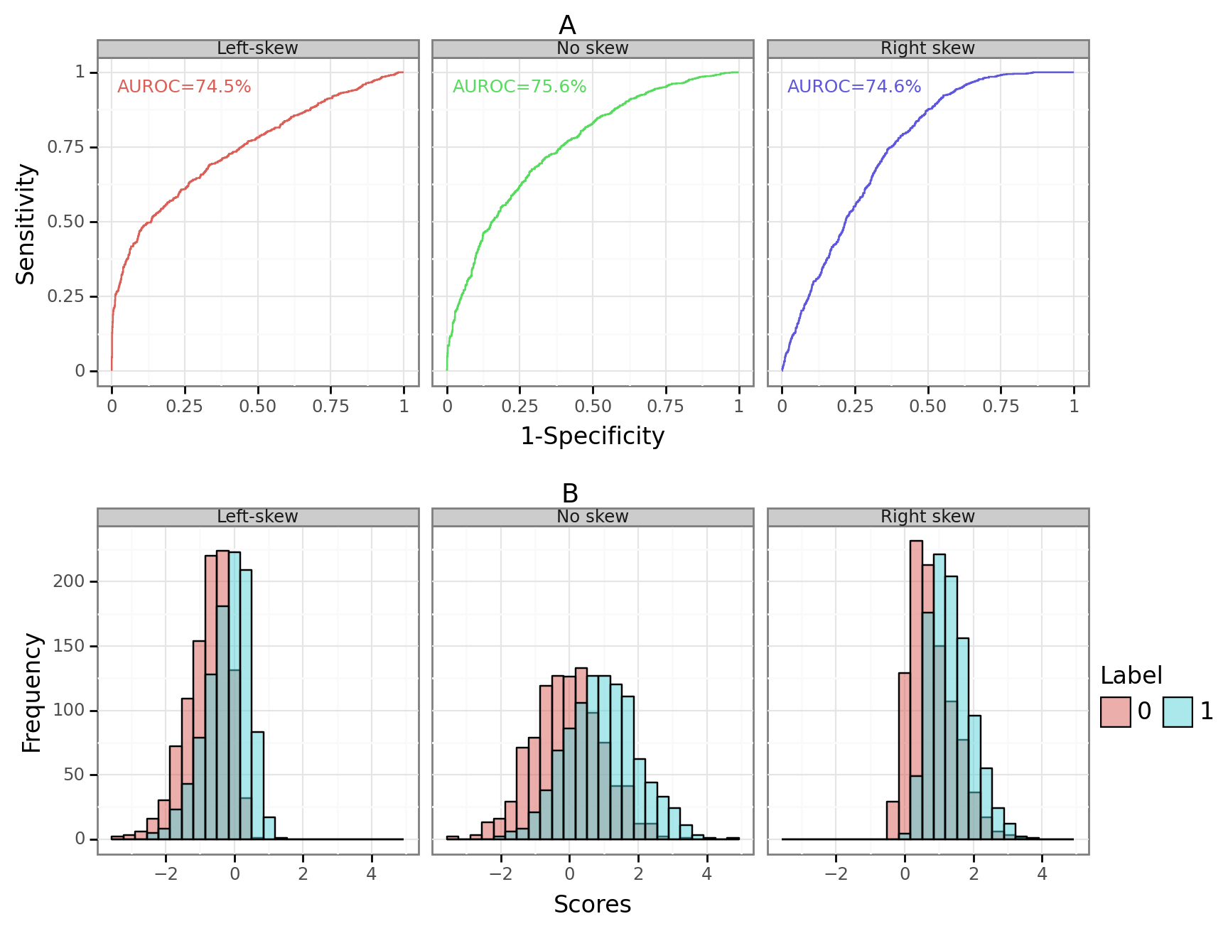
$n_0=n_1=1000$ for each class

$[\text{Left-skew}, \text{No-skew}, \text{Right-skew}]\sim SN([0.58,0.96,0.58],1,[-4,0,4])$

The empirical ROC curve should be treated as a random variable, with uncertainty occurring in the class-specific eCDFs \eqref{eq:emp_roc}. Figure 2 below shows the distribution of empirical ROC curves generated over 250 simulations. The ground truth ROC curve refers to the oracle value \eqref{eq:oracle_roc}. While the different draws of the data tend to centre around the true curve, there is substantial variation. In practice therefore, any realized ROC curve will provide a somewhat misleading representation of the actual TPR/FPR trade-off.

Figure 2: The ROC curve is a random variable

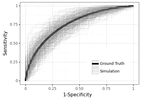
250 simulations; $\mu=1$, $n=100$, $n_1\sim \text{Bin}(n, 0.5)$, $n_0=n-n_1$

When one refers to picking a point on the ROC curve, one is actually referring to picking an operating threshold from a finite set of score values that corresponds to a specific empirical TPR/FPR combination. To see the implications of this random process, consider a classifier that always picks the point on the ROC curve that obtains 50% sensitivity. Figure 3A shows the different threshold choices that would be empirically chosen for the target of 50% sensitivity across 250 simulations. The empirically chosen operating threshold is often significantly above or below the oracle value, as Figure 2B shows. Whenever the empirical operating threshold is above (below) the oracle value, the expected sensitivity of the classifier will be lower (higher) than its true long-run value.

Figure 3: The operating threshold is a random variable

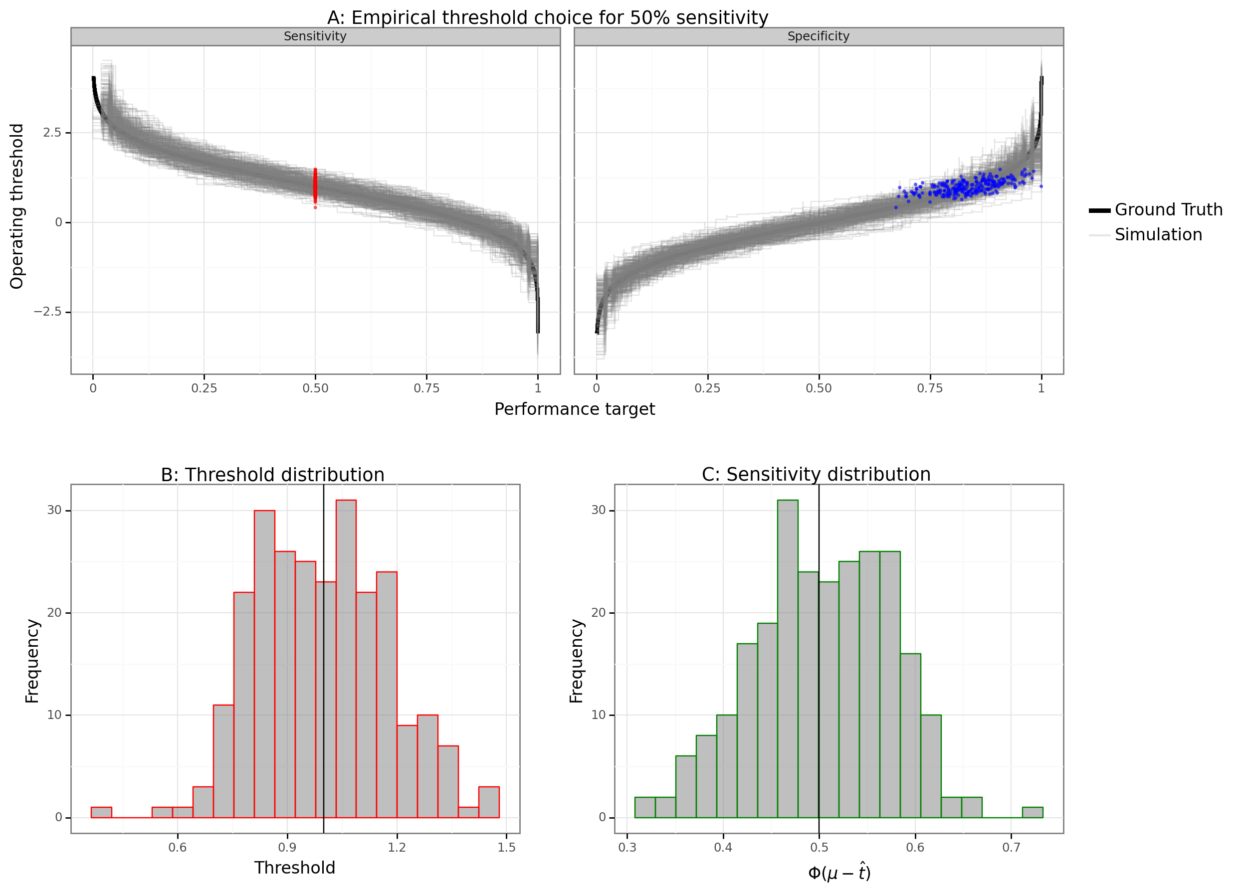
250 simulations; vertical lines show oracle values

$\mu=1$, $n=100$, $n_1\sim \text{Bin}(n, 0.5)$, $n_0=n-n_1$, $t^{*}_{0.5} = \mu + \Phi^{-1}(0.5) = 1$

Figure 3A also shows that when an empirically chosen operating threshold targets a high sensitivity or specificity, the variation and bias of the estimator increases. This is to be expected because the variance of order statistics grows the farther away they are from the median. Sample quantiles, while asymptotically consistent, can have quite a large bias for small sample sizes. Another problem with selecting high/low order statistics is that the size between observations is larger.[⁵] In summary, the empirical ROC curve is a random variable whose variation comes from the uncertainty between an operating threshold and the expected TPR/FPR.

(3) Probabilistic power analysis

The goal of a prospective trial is to establish that a classifier has at least some level performance.[⁶] For example, we might want to say that a classifier has at least 50% sensitivity and 60% specificity. Regardless of the distribution of the scores, the distribution of the predicted labels (\(z\)) will have a Bernoulli distribution. Since sensitivity and specificity are just averages of these Bernoulli distributed predicted labels, these performance measures will have binomial distribution.

\[\begin{align*} z_j &\sim \text{Bern}(\gamma_j) \\ \gamma_j &= P(s_j \geq t) \\ \text{sens}(y, z) &\sim n_1^{-1}\text{Bin}(n_1, \gamma_1) \\ \text{spec}(y, z) &\sim n_0^{-1}\text{Bin}(n_0, 1-\gamma_0) \\ \gamma_j &= \begin{cases} \Phi(\mu-t) & \text{ if } j = 1 \\ \Phi(-t) & \text{ if } j = 0 \end{cases} \end{align*}\]

Any binary classifier being evaluated in terms of sensitivity or specificity will have a test statistic that follows a binomial distribution. When \(n_0\) and \(n_1\) are large enough, this distribution will be approximately normal. To provide statistical evidence towards the claim that the sensitivity or specificity is at least \(\gamma_1\) and \(1-\gamma_0\), we can set a null hypothesis for each measure, with the goal of rejecting that null hypothesis in favour of the alternative.

\[\begin{align*} H_0&: \begin{cases} \gamma_1 \leq \gamma_{01} & \text{ if } j=1 \\ 1-\gamma_0 \leq 1-\gamma_{00} & \text{ if } j=0 \end{cases} \\ H_A&: \begin{cases} \gamma_1 > \gamma_{01} & \text{ if } j=1 \\ 1-\gamma_0 > 1-\gamma_{00} & \text{ if } j=0 \end{cases} \\ w &= \begin{cases} \frac{\hat{\gamma}_1 - \gamma_{01}}{\sigma_{01}} & \text{ if } j=1 \\ \frac{\gamma_{00}-\hat{\gamma}_0}{\sigma_{00}} & \text{ if } j=0 \end{cases} \tag{3}\label{eq:stat} \\ &\overset{a}{\sim} N(0,1) \hspace{1mm} \big| \hspace{1mm} H_0 \\ P(\text{Reject } H_0) &= P( w > c_\alpha ) \\ c_\alpha &= \Phi^{-1}(1-\alpha) \\ \hat{\gamma}_j &= n_j^{-1} \sum_{i=1}^{n_j} z_i \\ \sigma_{0j} &= \sqrt{\gamma_{0j}(1-\gamma_{0j}) / n_j} \end{align*}\]

If the operating threshold was set so that the conditionally expected value of the predicted labels matched the null hypothesis, \(P(s_j \geq t) = \gamma_{0j}\), then the test statistic \eqref{eq:stat} would have a standard normal distribution. The critical value (\(c_\alpha\)) is set so that the null hypothesis would be (erroneously) rejected (100\(\alpha\))% of the time when the null is true.

When the expected value of the performance measure is greater than the null hypothesis value (e.g. \(E(\hat\gamma_1) > \gamma_{0j}\)), then the alternative hypothesis is true. The probability of rejecting the null hypothesis when it is false is referred to as the power of a test. The type-II error of a test (\(\beta\)) is one less the power, and it is the probability of failing to reject the null when it is false. When the normal approximation holds from \eqref{eq:stat}, the type-II error can be analytical derived.

\[\begin{align*} \beta_j &= P(w < c_\alpha | H_A ) \\ &= \begin{cases} \Phi\Big( \frac{\sigma_{01} c_\alpha - [\gamma_1 - \gamma_{01}] }{\sigma_{A1}} \Big) & \text{ if } j=1 \\ \Phi\Big( \frac{\sigma_{00} c_\alpha - [\gamma_{00} - \gamma_0] }{\sigma_{A0}} \Big) & \text{ if } j=0 \end{cases} \tag{4}\label{eq:typeII} \\ \sigma_{Aj} &= \sqrt{\gamma_{j}(1-\gamma_{j}) / n_j} \end{align*}\]

There are two key parameters that determine the type-II error (and hence the power) of the statistical test seen in \eqref{eq:typeII}. The first is what is hereafter referred to as the “null hypothesis margin.” In the case of sensitivity, this is the spread between the actual TPR and the TPR under the null: \(\gamma_1 - \gamma_{01}\). For specificity, this is the spread between the FPR rate under the null, and what it is in reality: \(\gamma_{00} - \gamma_0\). The second is the sample size, which multiplies the null hypothesis margin by a factor of \(\sqrt{n_j}\). For a more elaborate breakdown of \eqref{eq:typeII}, see Section (3) from this previous post.

As Section (2) has made clear, plugging in \(\hat\gamma_j\) as an estimate for \(\gamma_j\) will provide a poor point estimate of the power as there is significant uncertainty around the long-run sensitivity/specificity for any empirical choice of \(t\). Instead of providing a point estimate of the power, we can draw from an approximate distribution of the classifier’s sensitivity and specificity, and then examine the distribution of the power estimates. The first approach, shown below, is to treat two performance measures as binomial distributions and sample around their point estimate. This amounts to a parametric bootstrap since we are ignoring the eCDF of the scores and directly sampling from an empirically informed parametric distribution.

\[\begin{align*} &\text{Parametric bootstrap} \\ \tilde{\text{sens}} &\sim \text{Bin}(n_1, \hat\gamma_1) \\ \tilde{\text{spec}} &\sim \text{Bin}(n_1, 1-\hat\gamma_0) \\ \tilde\beta_j &= \begin{cases} \Phi\Big( \frac{\sigma_{01} c_\alpha - [\tilde{\text{sens}} - \gamma_{01}] }{\tilde\sigma_{A1}} \Big) & \text{ if } j=1 \\ \Phi\Big( \frac{\sigma_{00} c_\alpha - [\tilde{\text{spec}} - \gamma_{00}] }{\tilde\sigma_{A0}} \Big) & \text{ if } j=0 \end{cases} \end{align*}\]

The second approach is to directly bootstrap the scores from the bottom-up and apply the bootstrapped performance measures directly into the power formula.

\[\begin{align*} &\text{Non-parametric bootstrap} \\ \tilde{s}_j &\sim \hat{F}_j \\ \tilde{\text{sens}} &= \sum_{i=1}^{n_1} I(\tilde{s}_{i1} \geq t) \\ \tilde{\text{spec}} &= \sum_{i=1}^{n_0} I(\tilde{s}_{i0} < t) \\ \tilde\beta_j &= \begin{cases} \Phi\Big( \frac{\sigma_{01} c_\alpha - [\tilde{\text{sens}} - \gamma_{01}] }{\tilde\sigma_{A1}} \Big) & \text{ if } j=1 \\ \Phi\Big( \frac{\sigma_{00} c_\alpha - [\tilde{\text{spec}} - \gamma_{00}] }{\tilde\sigma_{A0}} \Big) & \text{ if } j=0 \end{cases} \end{align*}\]

After one has obtained \(B\)-bootstrapped estimates of the power, \(\tilde\beta=[\tilde\beta_1, \dots, \tilde\beta_B]\), there are several approaches that can be used to calculate a CI around the point estimate \(\hat\beta\). I will refer readers to Section (2) of another post for more information about these methods. Figure 4 below shows a 95% CI as a function of the trial sample size, the null hypothesis margin, and the test set size (which is where the scores are drawn from).

Figure 4: Power uncertainty ranges

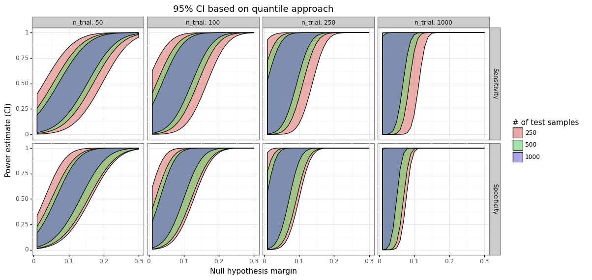
Uses the $[\alpha,1-\alpha]$ quantiles of the bootstrapped distribution

$\mu=1$, $E[n_1]=n/2$, $\alpha=0.05$

As the null hypothesis margin grows, the power estimate increases and the uncertainty around it declines. For small margins, the uncertainty is also reduced, with a low upper-bound on the possible power. Figure 4 shows that the uncertainty around the power is actually at its peak for medium ranges of the null hypothesis margin. This is to be expected since variation in the sensitivity or specificity above the mean will suggest a high power, whilst deviations below the mean will imply low power. When the sample size of the scores increases (test size), the CIs shrink as there is less variation in the simulated draws of sensitivity and specificity.

We can now re-examine the empirical operating threshold/performance measure curve seen in Figure 3A in terms of a probabilistic power analysis. Figure 5 below provides a visual summary of how high power is expected to be relative to the the empirical trade-off curve. When the oracle operating threshold value exceeds the empirical one, the point estimate of the power will be conservative. When the empirical line exceeds the oracle, then the point estimate of the power will be optimistic. The goal of these CIs is to have the lower- and upper-bounds capture the oracle value at a certain statistical frequency.

Figure 5: Null hypothesis margin and power ranges

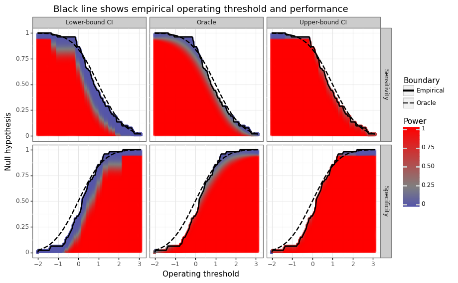
Uses the $[\alpha,1-\alpha]$ quantiles of the bootstrapped distribution

$E(n_1)=50$, $n=100$, $n_1^{\text{trial}}=n_0^{\text{trial}}=50$

(4) Simulation results

Before assessing the quality of the bootstrapped CIs, it is worth checking in on the quality of the power estimates. Recall that the test statistics for sensitivity and specificity seen in \eqref{eq:stat} and their corresponding analytical power (type-II error) formulation \eqref{eq:typeII} were based on a normal approximation of a binomial distribution. In other words, we should check that the expected power lines up with the empirical null hypothesis rejection rate: i.e. \(P(w > c_\alpha)\). Figure 6 below shows relationship between the expected power (using the oracle sensitivity/specificity) and the empirical rejection rate of the null hypothesis.

Figure 6: Power calibration

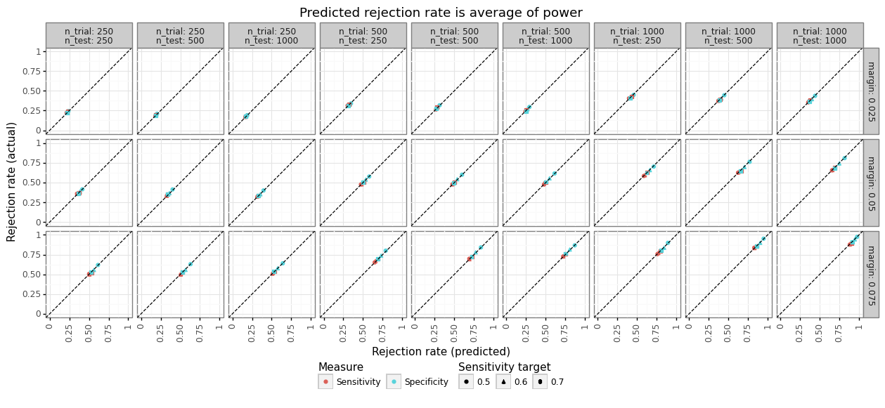
2500 simulations, uses oracle power

$\mu=1$, $E[n_1]=n/2$, $\alpha=0.05$

The simulations were done over different sample sizes for the test set and trial set, oracle null hypothesis margins, and empirical sensitivity targets. As Figure 6 makes clear, assuming one knew the oracle sensitivity, the power (type-II error) estimate from \eqref{eq:typeII} is a highly accurate approximation. Over these same simulations, we can also compare the parametric and non-parametric bootstrapped CI approaches in terms of their coverage.

Figure 7: Bootstrapping methods and power coverage

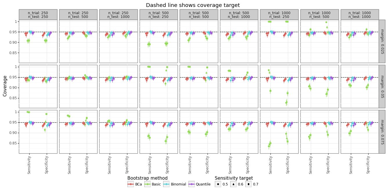
Margin is set relative to sensitivity target

2500 simulations, 1000 bootstrap iterations, four bootstrapping CI approaches

$\mu=1$, $E[n_1]=n/2$, $\alpha=0.05$

Figure 7 shows the empirical coverage compared to the nominal target of 95% by the different approaches. The three bootstrapping approaches that use quantiles all work relatively well: the quantile, the bias-corrected and accelerated (BCa), and the binomial (parametric) method. The uncertainty bars are the variation range one would expected for 2500 simulations. Most of the time the coverage is either statistically indistinguishable from its nominal target, or very close. The basic bootstrapping method, which only uses the standard error of the bootstrapped samples, often under- or over-shoots its nominal target. Basic bootstraps tend to work poorly on non-symmetric distributions.

(5) Conclusion

This post has provided a novel framework for designing a statistical trial for a binary classifier when the goal is to establish performance bounds on sensitivity and specificity simultaneously. Unlike validating a single performance measure, a conservative estimate of the operating threshold cannot be chosen due to its conflicting implications for the TPR and TNR. By simulating the variation in the class-specific scores, and keeping the operating threshold fixed, we can study the range of likely performance measure values. A two-sided confidence interval of the subsequent power of the prospective trial can be constructed which has coverage properties close to its expected level. Because the binomial method is the computationally cheapest approach, and its performance is on par with the non-parametric bootstrapping methods, I recommend using this method when doing inference.

To conclude, let’s see how we can use these techniques on a real world dataset. I trained a simple logistic regression model on the a Diabetes dataset by discretizing the label at the median point. The training and test set were randomly split 50/50. The scores were logit-transformed test set model probabilities. For three operating threshold points (-2, 0, 2), the null hypothesis was set to the empirical sensitivity/specificity at that point, less some margin (0%, 10%, and 20%). The future trial dataset was assumed to have 400 observations, with an equal split between the positive and negative classes.

Figure 8 below shows the empirical operating threshold curve and the associated power CIs. By setting the null hypothesis to 20% below the empirical value for both performance measures, the trial is almost guaranteed to succeed. When the null is set to the empirical value, then the power ranges from roughly 0-100%. This indicates that there is sufficient variation around the point estimate of the performance measure to be unsure of any subsequent trial. When the margin is 10%, the CIs have a varying interval length. When the empirical sensitivity or specificity values are high at around 95% (i.e. a low/high threshold, respectively), then the CI interval lengths are fairly tight. This is to be expected as the variance of a binomial distribution decreases for probability values close to zero or one. However, when the performance measure values are more moderate, then even a 10% margin is associated with significant variation in the power estimates. In other words, the impact of a given null hypothesis margin will vary depending on the baseline level of the performance measure.

Figure 8: Trial power range on the Diabetes dataset

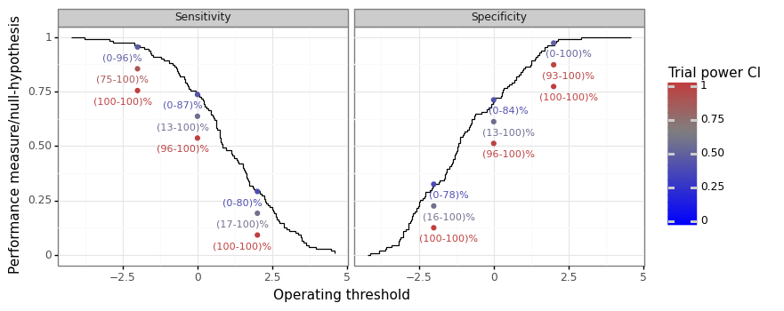
Binomial method on 1000 bootstrap iterations

$n_1=110$, $n_0=111$, $n_1^{\text{trial}}=n_0^{\text{trial}}=200$, $\alpha=0.05$

---