
sntn: A package to support data carving
This post accompanies the release of the sntn package, which implements a scipy-like class for doing inference on a sum of a normal and a trunctated normal (SNTN) distribution (see Kim (2006) and Arnold (1993)). I’ve written about this distribution before.
The SNTN distribution can be used in a variety of situations including data carving (a type of post-selection inference), situations where a filtering process is applied, as well as two-stage hypothesis testing. The arXiv paper, “A parametric distribution for exact post-selection inference with data carving” makes extensive use of this package.
Formally, if \(X_1 \sim N(\mu_1, \tau_1^2)\) and \(X_2 \sim \text{TN}(\mu_2, \tau_2^2, a, b)\), then \(Z = c_1 X_1 + c_2 X_2\), \(c_i \in \mathbb{R}\), is said to follow an SNTN distribution denoted as either \(\text{SNTN}(\mu_1, \tau_1^2, \mu_2, \tau_2^2, a, b, c_1, c_2)\overset{d}{=}\text{SNTN}(\theta_1, \sigma_1^2, \theta_2, \sigma_2^2, \omega, \delta)\) where \(\theta_1=\sum_i c_i\mu_i\), \(\sigma_1^2=\sum_i c_i^2\tau_i^2\), \(\theta_2=\mu_2\), \(\sigma_2^2=\tau_2^2\), \(m_j(x)=(x-\theta_x)/\sigma_x\), \(\omega=m_2(a)=(a-\theta_2)/\sigma_2\), and \(\delta=m_2(b)=(b-\theta_2)/\sigma_2\).
Inference for the SNTN distributions ends up being computationally scalable since the cdf (\(f\)) has a closed form solution, and the CDF (\(F\)) can be calculated using the CDF of two bivariate normal distributions with correlation \(\rho\).
\[\begin{align*} f_{\theta,\sigma^2}^{\omega,\delta}(z) &= \frac{\phi(m_1(z))[\Phi(\gamma\delta -\lambda m_1(z)) - \Phi(\gamma\omega -\lambda m_1(z))]}{\sigma_1[\Phi(\delta)-\Phi(\omega)]} \\ F_{\theta,\sigma^2}^{\omega,\delta}(z) &= \frac{B_\rho(m_1(z),\delta) - B_\rho(m_1(z),\omega)}{\Phi(\delta)-\Phi(\omega)} \\ \rho&=c_2\sigma_2/\sigma_1 \\ \lambda &= \rho/\sqrt{1-\rho^2} \\ \gamma &= \lambda/\rho \end{align*}\]This post will show to use the sntn package to do data carving, a type of post-selection inference (PoSI), for the lasso and marginal screening algorithms.
Background
In post-selection inference (PoSI), we want to run a classic linear regression on a subset of features that have been selected by some algorithm. The statistical quantity of interest is a one-dimensional term \(\eta_j^T g=\beta_j^0\), which is the inner product of a row from the matrix \([(X^TX)^{-1}X^T]_{j:}\) and the signal component of the response for a model of additive error: \(y=g(x)+e\), \(e\sim N(0,\sigma^2 I_n)\), where \(g\) is usually assumed to be linear. For example, if the Lasso is run for a fixed value of \(\lambda\), then we could consider running a linear regression on only those coordinates which it selected non-zero coefficients for.
\[M = \{j: \beta^{\text{lasso}}_\lambda \neq 0\} \subset \{1, \dots, p\}\]Recent research has shown that for the Lasso, and other algorithms (like marginal screening or forward stepwise regression), the selection event \(M\) can be shown to be in bijection with a polyhedral constraints on \(y\) which leads to a trunctated normal distribution.
\[\hat\beta^{\text{PoSI}}_j = \eta^T_{M_j}y \sim \text{TN}(\beta_j^{M}, \sigma^2_M \|\eta_{M_j}\|^2_2, V^{-}(y), V^{+}(y))\]If this estimator is combined with another portion of data that was unused in the Lasso alogithm,
\[\hat\beta^{\text{OLS}}_j = \eta^T_{M_j}y \sim N(\beta_j^{M}, \sigma^2_M \|\eta_{M_j}\|^2_2)\]Then the (weighted) sum of these two coefficients will follow an SNTN distribution, where \(w_A\) and \(w_B\) are the relative sample sizes which sum to one.
\[\begin{align*} \hat\beta^{\text{carve}}_j &= w_A \hat\beta^{\text{OLS}}_j + w_B \hat\beta^{\text{PoSI}}_j \\ &\sim SNTN(\beta_j^{M}, \sigma^2_M \|\eta^A_{M_j}\|^2_2, \beta_j^{M}, \sigma^2_M \|\eta^B_{M_j}\|^2_2, w_A, w_B) \end{align*}\]TLDR
While this notebook will provide a deeper dive on how to obtain valid inference with the SNTN distribution for data carving-PoSI for both the lasso and marginal screening, wrappers have been built into the package to do a lot of the leavy lifting under the hood. This first TLDR section will show how to use them directly, while latter sections will go into more detail about what is happening behind the scenes.
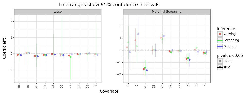
The Wisconsin Breast Cancer dataset will be used (\(n=569\), \(p=30\)). A type-1 error rate of 5% is set with alpha. The first code block shows to obtain inferene using the lasso and marginal screen wrappers.
# Load external packages
import numpy as np
import pandas as pd
import plotnine as pn
from scipy.stats import norm
from glmnet import ElasticNet
from sklearn.datasets import load_breast_cancer
from sklearn.model_selection import train_test_split
# Load SNTN utilities
from sntn.dists import nts, tnorm
from sntn.posi import lasso, marginal_screen

# For reproducability
seed = 1

# Checking numerical stability of solutions
kkt_tol = 5e-3

# Set up null-hypothesis testing
alpha = 0.05
null_beta = 0

# Load dataset
X, y = load_breast_cancer(return_X_y=True)
cn_X = load_breast_cancer().feature_names
n, p = X.shape

# Specify hyperparameters
pct_split = 0.50  # Percent to use for inference
lamb_fix = 1e-2  # lambda value for Lasso
k = 10  # Top-k correlated variables to select

# Run the PoSI-Lasso
wrapper_lasso = lasso(lamb_fix, y, X, frac_split=pct_split, seed=seed)
sigma2 = wrapper_lasso.ols_split.sig2hat
wrapper_lasso.run_inference(alpha, null_beta, sigma2)

# Run the PoSI-Marginal Screener
wrapper_margin = marginal_screen(k, y, X, frac_split=pct_split, seed=seed)
sigma2 = wrapper_margin.ols_split.sig2hat
wrapper_margin.run_inference(alpha, null_beta, sigma2)
# Combine results
res_lasso = pd.concat(objs=[wrapper_lasso.res_screen.assign(inf='Screening'),
                            wrapper_lasso.res_split.assign(inf='Splitting'),
                            wrapper_lasso.res_carve.assign(inf='Carving')], axis=0)
res_lasso.insert(0, 'mdl', 'Lasso')
res_margin = pd.concat(objs=[wrapper_margin.res_screen.assign(inf='Screening'),
                             wrapper_margin.res_split.assign(inf='Splitting'),
                             wrapper_margin.res_carve.assign(inf='Carving')], axis=0)
res_margin.insert(0, 'mdl', 'Marginal Screening')
res_posi = pd.concat(objs=[res_lasso, res_margin], axis=0).reset_index(drop=True)
res_posi = res_posi.assign(is_sig = lambda x: x['pval'] < alpha)
# Plot
posd = pn.position_dodge(0.5)
gg_posi = (pn.ggplot(res_posi, pn.aes(x='cidx.astype(str)',y='bhat',color='inf',alpha='is_sig')) +
            pn.theme_bw() +
            pn.facet_wrap('~mdl',scales='free') +
            pn.geom_point(size=2,position=posd) +
            pn.geom_hline(yintercept=0,linetype='--') +
            pn.geom_linerange(pn.aes(ymin='lb.clip(lower=-100)',ymax='ub.clip(upper=100)'),position=posd) +
            pn.ggtitle(f'Line-ranges show {100*(1-alpha):0.0f}% confidence intervals') +
            pn.labs(x='Covariate',y='Coefficient') +
            pn.scale_color_discrete(name='Inference') +
            pn.scale_alpha_manual(name=f'p-value<{alpha}',values=[0.3,1]) +
            pn.theme(axis_text_x=pn.element_text(angle=90),subplots_adjust={'wspace': 0.25}))
gg_posi
Deep dive: Data-split
While the posi wrappers handle the data splitting under the hood, the rest of this post will show how to replicate these results from scratch. A 50/50% split will be used, such that half of the data will go towards fitting the Lasso and the other half will be used for inference.
Group A will refer to the inference set (unbiased) and group B refers to the screening set which will be used by the Lasso or marginal sceener.
X_B, X_A, y_B, y_A = train_test_split(X, y, test_size=pct_split, random_state=seed)
n_A, n_B = len(y_A), len(y_B)
w_A, w_B = n_A/n, n_B/n
# Normalize B (which will go into algorithms)
mu_A = X_A.mean(0)
mu_B = X_B.mean(0)
se_B = X_B.std(0,ddof=1)
Xtil_B = (X_B - mu_B) / se_B
# Put A on the same scale as B so the coefficients have the same intepretation, but de-mean so we don't need to worry about intercept
Xtil_A = (X_A - mu_A) / se_B

# De-mean y so we don't need to fit intercept
ytil_A = y_A - y_A.mean()
ytil_B = y_B - y_B.mean()
Deep dive: Lasso-PoSI
Readers are encouraged to read Lee et al. (2016), hereafter Lee16 for a derivation and proof and derivation of many of the terms that will be used.
# (i) Run the Lasso for some fixed value of lambda
lamb_path = np.array([lamb_fix*1.01, lamb_fix])  # ElasticNet wants >=2 values
mdl_lasso = ElasticNet(alpha=1, n_splits=0, standardize=False, lambda_path=lamb_path, tol=1e-20)
mdl_lasso.fit(Xtil_B, ytil_B)
bhat_lasso = mdl_lasso.coef_path_[:,1]
M_lasso = bhat_lasso != 0
cn_lasso = cn_X[M_lasso]
X_B_M = Xtil_B[:,M_lasso].copy()
# Check KKT conditions
kkt_lasso = np.abs(Xtil_B.T.dot(ytil_B - Xtil_B.dot(bhat_lasso)) / n_B)
err_kkt = np.max(np.abs(kkt_lasso[M_lasso] - lamb_fix))
assert err_kkt < kkt_tol, 'KKT conditions not met'
assert np.all(lamb_fix > kkt_lasso[~M_lasso]), 'KKT conditions not met'
n_sel = M_lasso.sum()
print(f'Lasso selected {n_sel} of {p} features for lambda={lamb_fix} (KKT-err={err_kkt:0.5f})')

# (ii) Run OLS on the screening portion
igram_B_M = np.linalg.inv(np.dot(X_B_M.T, X_B_M))
eta_B_M = np.dot(X_B_M, igram_B_M)
bhat_B = np.dot(eta_B_M.T, ytil_B)

# (iii) Run inference on the classical held-out portion
X_A_M = Xtil_A[:,M_lasso].copy()
igram_A_M = np.linalg.inv(np.dot(X_A_M.T, X_A_M))
eta_A_M = np.dot(X_A_M, igram_A_M)
bhat_A = np.dot(eta_A_M.T, ytil_A)

# (iv) Use held-out portion to estimate variance of the error
resid_A = ytil_A - np.dot(X_A_M, bhat_A)
sigma2_A = np.sum(resid_A**2) / (n_A - (n_sel+1))
tau21 = sigma2_A * np.sum(eta_A_M**2,0)
Lasso selected 10 of 30 features for lambda=0.01 (KKT-err=0.00000)
Following Lee’s paper, we’ll follow equations (4.8) to (5.6), using only A1/b1 because we are only considering partial inference.
# (v) Calculate the polyhedral constraints
sign_M = np.diag(np.sign(bhat_lasso[M_lasso]).astype(int))
A = -np.dot(sign_M, eta_B_M.T)
# Note, that lambda is multiplied by n_B since the solution below solves for the non-normalized version
b = -n_B * lamb_fix * np.dot(sign_M, np.dot(igram_B_M, sign_M.diagonal()))
# Check for constraint error
assert  np.all(A.dot(ytil_B) <= b), 'Polyhedral constraint not met!'

# (vi) Calculate the truncated normal values (4.8 to 5.6 for Lee's paper, using only A1/A2)
tau22 = sigma2_A * np.sum(eta_B_M**2,0)
D = np.sqrt(tau22 / sigma2_A)
V = eta_B_M / D
R = np.squeeze(np.dstack([np.dot(np.identity(n_B) - np.outer(V[:,j],V[:,j]),ytil_B)  for j in range(n_sel)]))
AV = np.dot(A, V)
AR = A.dot(R)
nu = (b.reshape([n_sel,1]) - AR) / AV
idx_neg = AV < 0
idx_pos = AV > 0
a = np.max(np.where(idx_neg, nu, -np.inf),0) * D
b = np.min(np.where(idx_pos, nu, +np.inf),0) * D
assert np.all(b > a), 'expected pos to be larger than neg'
We can now set up all of the specific distributions.
# Signs can be used to determine direction of hypothesis test
is_sign_neg = np.sign(bhat_lasso[M_lasso])==-1

# (i) PoSI with the Lasso
dist_tnorm = tnorm(null_beta, tau22, a, b)
pval_tnorm = dist_tnorm.cdf(bhat_B)
pval_tnorm = np.where(is_sign_neg, pval_tnorm, 1-pval_tnorm)
res_tnorm = pd.DataFrame({'mdl':'Screening','cn':cn_lasso,'bhat':bhat_B, 'pval':pval_tnorm})
res_tnorm = pd.concat(objs=[res_tnorm, pd.DataFrame(dist_tnorm.conf_int(bhat_B, alpha),columns=['lb','ub'])],axis=1)

# (ii) OLS on inference set
dist_norm = norm(loc=null_beta, scale=np.sqrt(tau21))
pval_norm = dist_norm.cdf(bhat_A)
pval_norm = np.where(is_sign_neg, pval_norm, 1-pval_norm)
res_norm = pd.DataFrame({'mdl':'Splitting','cn':cn_lasso, 'bhat':bhat_A, 'pval':pval_norm})
res_norm = pd.concat(objs=[res_norm, pd.DataFrame(np.vstack(norm(bhat_A, np.sqrt(tau21)).interval(1-alpha)).T,columns=['lb','ub'])],axis=1)

# (iii) Data carving on both
bhat_wAB = w_A*bhat_A + w_B*bhat_B
dist_sntn = nts(null_beta, tau21, null_beta, tau22, a, b, w_A, w_B, fix_mu=True)
pval_sntn = dist_sntn.cdf(bhat_wAB)
pval_sntn = np.where(is_sign_neg, pval_sntn, 1-pval_sntn)
res_sntn = pd.DataFrame({'mdl':'Carving','cn':cn_lasso,'bhat':bhat_wAB, 'pval':pval_sntn})
res_sntn = pd.concat(objs=[res_sntn, pd.DataFrame(np.squeeze(dist_sntn.conf_int(bhat_wAB, alpha)),columns=['lb','ub'])],axis=1)
This should align to the results we find the wrapper
print(np.max(np.abs(res_sntn['pval'] - res_lasso.loc[res_lasso['inf'] == 'Carving','pval'])))
1.2656542480726785e-14
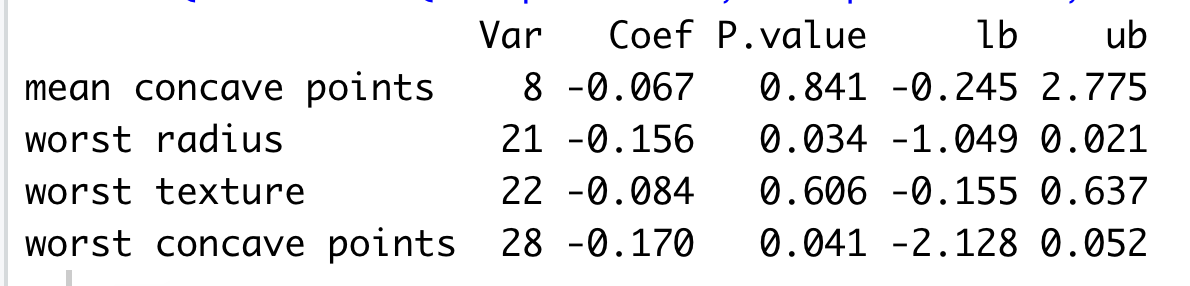
Comparing to R
As the wisconsin_replicate.R file shows, the python wrapper can get close to the same results (where the confidence intervals differ slightly due to the different root finding routines in effect).
ytil = y - y.mean()
xtil = (X - X.mean(0)) / X.std(0, ddof=0)
inf2R = lasso(0.1, y, X, frac_split=0)
inf2R.run_inference(alpha, null_beta, 1.0, run_split=False, run_carve=False)
inf2R.res_screen.round(3)
| cidx | bhat | pval | lb | ub | |
|---|---|---|---|---|---|
| 0 | 7 | -0.067 | 0.841 | -0.243 | 2.774 |
| 1 | 20 | -0.156 | 0.034 | -1.049 | 0.020 |
| 2 | 21 | -0.084 | 0.606 | -0.155 | 0.637 |
| 3 | 27 | -0.170 | 0.041 | -2.127 | 0.051 |
(3) Marginal screening
Following the same recipe for the Lasso, this time we will follow Lee & Taylor (2014), hereafter Lee14 to break down step-by-step what is happening under the hood for the posi.marginal_screen wrapper.
# (i) Run marginal screening and find the top-k features
k = 10
Xty = Xtil_B.T.dot(ytil_B)
aXty = np.abs(Xty)
cidx_ord = pd.Series(aXty).sort_values().index.values
cidx_k = cidx_ord[-k:]
S_margin = np.sign(Xty[cidx_k])
assert np.all(np.sign(Xty) == np.sign([np.corrcoef(Xtil_B[:,j],ytil_B)[0,1] for j in range(p)])), 'Inner product should align with signs of Pearson correlation'
M_margin = np.isin(np.arange(p), cidx_k)
cn_margin = cn_X[M_margin]
X_B_M = Xtil_B[:,M_margin].copy()
# Check KKT
assert np.all(np.atleast_2d(aXty[M_margin]).T > aXty[~M_margin]), 'KKT for marginal screening not met'

# (ii) Run OLS on the screening portion
igram_B_M = np.linalg.inv(np.dot(X_B_M.T, X_B_M))
eta_B_M = np.dot(X_B_M, igram_B_M)
bhat_B = np.dot(eta_B_M.T, ytil_B)

# (iii) Run inference on the classical held-out portion
X_A_M = Xtil_A[:,M_margin].copy()
igram_A_M = np.linalg.inv(np.dot(X_A_M.T, X_A_M))
eta_A_M = np.dot(X_A_M, igram_A_M)
bhat_A = np.dot(eta_A_M.T, ytil_A)

# (iv) Use held-out portion to estimate variance of the error
resid_A = ytil_A - np.dot(X_A_M, bhat_A)
sigma2_A = np.sum(resid_A**2) / (n_A - (k+1))
tau21 = sigma2_A * np.sum(eta_A_M**2,0)

# (v) Calculate the polyhedral constraints
partial = np.identity(p)
partial = partial[~M_margin]
partial = np.vstack([partial, -partial])
Now we ready to calculate the the polyhedral constraints (see equations (5)-(8) from Lee14).
# Create an array with all zeros
A = np.zeros(partial.shape + (k,))
# Set specified column indices to opposite sign of the coeficient
for i, idx in enumerate(cidx_k):
    A[:, idx, i] = -S_margin[i]
A = np.vstack([A[...,j] for j in range(k)])
A += np.tile(partial,[k,1])
A = A.dot(Xtil_B.T)
# Check for constraint error
Ay = A.dot(ytil_B.reshape([n_B,1]))
assert  np.all(Ay <= 0), 'Polyhedral constraint not met for marginal screening!'

# (vi) Calculate the truncated normal values
tau22 = sigma2_A * np.sum(eta_B_M**2,0)
# See equation (6) - sigma2 will cancel out with tau22 when normalized
alph_num = sigma2_A * np.dot(A, eta_B_M)
alph = alph_num / tau22
ratio = -Ay/alph + np.atleast_2d(bhat_B)
idx_neg = alph < 0
idx_pos = alph > 0
a = np.max(np.where(alph < 0, ratio, -np.inf), axis=0)
b = np.min(np.where(alph > 0, ratio, +np.inf), axis=0)
assert np.all(b > a), 'expected pos to be larger than neg'
As before, we can use the custom distribution classes to get the inference under the null hypothesis.
is_sign_neg = S_margin==-1

# (i) PoSI with the Lasso
dist_tnorm = tnorm(null_beta, tau22, a, b)
pval_tnorm = dist_tnorm.cdf(bhat_B)
pval_tnorm = np.where(is_sign_neg, pval_tnorm, 1-pval_tnorm)
res_tnorm = pd.DataFrame({'mdl':'Screening','cn':cn_margin,'bhat':bhat_B, 'pval':pval_tnorm})
res_tnorm = pd.concat(objs=[res_tnorm, pd.DataFrame(dist_tnorm.conf_int(bhat_B, alpha),columns=['lb','ub'])],axis=1)

# (ii) OLS on inference set
dist_norm = norm(loc=null_beta, scale=np.sqrt(tau21))
pval_norm = dist_norm.cdf(bhat_A)
pval_norm = np.where(is_sign_neg, pval_norm, 1-pval_norm)
res_norm = pd.DataFrame({'mdl':'Splitting','cn':cn_margin, 'bhat':bhat_A, 'pval':pval_norm})
res_norm = pd.concat(objs=[res_norm, pd.DataFrame(np.vstack(norm(bhat_A, np.sqrt(tau21)).interval(1-alpha)).T,columns=['lb','ub'])],axis=1)

# (iii) Data carving on both
bhat_wAB = w_A*bhat_A + w_B*bhat_B
dist_sntn = nts(null_beta, tau21, null_beta, tau22, a, b, w_A, w_B, fix_mu=True)
pval_sntn = dist_sntn.cdf(bhat_wAB)
pval_sntn = np.where(is_sign_neg, pval_sntn, 1-pval_sntn)
res_sntn = pd.DataFrame({'mdl':'Carving','cn':cn_margin,'bhat':bhat_wAB, 'pval':pval_sntn})
res_sntn = pd.concat(objs=[res_sntn, pd.DataFrame(np.squeeze(dist_sntn.conf_int(bhat_wAB, alpha)),columns=['lb','ub'])],axis=1)
This should give us the same inference as the wrapper
print(np.max(np.abs(res_sntn.sort_values('bhat')['pval'].values - res_margin.loc[res_margin['inf'] == 'Carving'].sort_values('bhat')['pval'].values)))
4.2732484217822275e-13